1 Introduction

The iterative method to the large sparse 2×2 block linear system of equations

is considered,where the matrix A is m × m symmetric positive definite (SPD),the matrix B is m × n and has a full column rank,i.e.,rank (B) = n,vectors x,p ∈ R^m ,vectors y,q ∈ Rⁿ ,and superscript T stands for the transpose. Under these assumptions,the above linear system has a unique solution. The linear system (1) is important for many different applications of science computing ^{[1, 2, 3, 4]} ,such as fluid dynamics,the finite element method for solving the Navier-Stokes equation,constrained optimization,constrained or generalized least squares problems,image processing,and linear elasticity.

Since the above problem is large and sparse,the iterative methods for solving (1) are effective because of storage requirements and preservation of sparsity. The well-known successive overrelaxation-like (SOR) ^[5] and accelerated over-relaxation (AOR) ^[6] methods are simple iterative methods,which are popular in engineering applications. The difficulty for the SOR and AOR methods is the singularity of the block diagonal part of the coefficient matrix of the system (1). Recently,there have been several proposals ^{[7, 8, 9, 10, 11, 12]} for generalizing the SOR method for the above system. However,the most practical and important generalization of the SOR method is the SOR-like method given by Golub et al. ^[7] . The SOR-like method is more closely related to the format of the normal SOR splitting as follows:

and the SOR-like method is defined by the normal SOR procedure as

These motivate us to consider the following splitting form to the above system: where Q is a nonsingular and symmetric matrix. If we let then the modified SOR-like (MSOR-like) method can be defined by the following scheme: The above MSOR-like method involves one parameter ω and one preconditioning matrix Q. It is expected that by a proper choice of the parameter,the MSOR-like has a faster convergence rate than that of the well-known SOR-like method ^[8] and modified symmetric SOR-like (MSSORlike) method ^[10] in certain case. Note that Since the matrix A is SPD,and the matrix Q is nonsingular,we have

if and only if

In Section 2,we discuss the convergence analysis of the MSOR-like method,and in Section 3,we derive the convergence domain. In Section 4,the optimum for the MSOR-like are given. In Section 5,a numerical example is given to show the effectiveness of the MSOR-like method. 2 Basic functional equation and lemmas

If we let M_ω be the iteration matrix of the MSOR-like method and note that

then it can be shown that where _ωsatisfies (6). Firstly,we note that if_ω = 0,then

Thus,the MSOR-like method will diverge in this case. Therefore,from now on,we always assume that _ω ≠ 0 and _ω ≠ 2.

If we let λ be an eigenvalue of M_ω and (u,v) ^T be the corresponding eigenvector,we have

which is equivalent to

Lemma 2.1If λ is an eigenvalue of M_ω ,then λ ≠ 1.

Proof If λ = 1,and the associated eigenvector is (u,v)^T ,then following from (9) and ω ≠ 0,we have

resulting in Q ⁻¹ B ^T A ⁻¹ B_v = 0. Since Q⁻¹B^TA⁻¹B is nonsingular,we have that v = 0. It follows from (10) that u = 0. This contradicts to (u,v)^T ,which is an eigenvector of the iteration of M_ω . Hence,λ ≠ 1,concluding the proof.

Lemma 2.2 If m > n,then λ = 1 − ω ≠ 0 is an eigenvalue of M_ω at least with multiplicity of m − n. If m = n,then λ = 1 − ω ≠ 0 is not an eigenvalue of M_ω .

Proof If λ = 1 − ω ≠ 0 is an eigenvalue of M_ω ,then there exists a nonzero vector (u,v)^T so that they satisfy the system (8) with λ = 1 − ω ≠ 0. Therefore,by the system (9) and ω ≠ 0, we have

Since the matrix B has a full column rank,the above system is equivalent to

Since B^T∈ Rⁿ×m ,and rank ( B^T ) = n. If m > n,Q^-1B^Tu = 0 has m−n (> 0) independent nonzero solutions; if m = n,Q^-1B^Tu = 0 has no nonzero solution. Thus,λ = 1 − ω ≠ 0 is not only an eigenvalue of M_ω ,but also an eigenvalue with multiplicity of m − n if m > n,and λ = 1 − ω ≠ 0 is not an eigenvalue of M_ω if m = n,concluding the proof of Lemma 2.2.

Theorem 2.1 Let M_ω be the iteration matrix of the MSOR-like method. Then,

(i) λ = 1 − ω ≠ 0 is an eigenvalue of M_ω ,if m > n.

(ii) For any eigenvalue λ (λ ≠ 1 − ω) of M_ω ,there is an eigenvalue µ of Q⁻¹B^TA⁻¹B so that λ and ω satisfy the following functional equation:

(iii) For any eigenvalue µ of Q⁻¹B^TA⁻¹B,if λ is different from 1 − ω and 1,and µ and ω satisfy the above functional equation,then λ is an eigenvalue of M_ω .

Proof The conclusion (i) of Theorem 2.1 comes from Lemma 2.2.

For the conclusion (ii),we let λ ≠ 1 − ω be the eigenvalue of M_ω ,and (u,v)^T be the associated eigenvector. Then,they satisfy the system (9). Thus,we have

Since λ ≠ 1 − ω,λ ≠ 1 by Lemma 2.1,and v ≠ 0 by the note after Lemma 2.2,there is an eigenvalue µ of Q⁻¹B^TA⁻¹B satisfying the equation µv = Q⁻¹B^TA⁻¹Bv. Therefore,(12) is equivalent to (11),concluding the proof of the conclusion (ii).

For the conclusion (iii),we let u,v be the eigenvalue and associated eigenvector of the matrix Q⁻¹B^TA⁻¹B. Therefore,we have Q⁻¹B^TA⁻¹Bv = µv. By the conditions of the theorem,(12) holds. If we let

then it follows from (12) that the system (9) holds,which is equivalent to the system (9).

Thus,λ is an eigenvalue of M_ω ,since (u,v)^T is nonzero.

Corollary 2.1 If we let ρ(M_ω ) be the spectral radius of the MSOR-like iteration matrix M_ω and m > n,then we have ρ(M_ω ) > |1 − ω|.

Note that by the above corollary,the necessary condition for the convergence of the MSORlike method when m > n is

Lemma 2.3 ^[5] Both roots of the real quadratic equation λ² − bλ + c = 0 are less than one in modulus if and only if |c| < 1 and |b| < 1 + c. 3 Convergence analysis

From now on,we always assume that λ and µ are eigenvalues of the iteration matrix M_ω of the MSOR-like method and the matrix Q⁻¹B^TA⁻¹B,respectively. We also assume that the parameter ω satisfies the inequality (13). Thus,no matter 1 − ω is an eigenvalue of M_ω or not,it does not affect the convergence property of the MSOR-like method. Therefore,the MSOR-like method converges if and only if for any eigenvalue µ,the solution λ of (11) is less than unity in modulus. Then,(11) is equivalent to

where

Then,we have the following results.

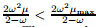
Theorem 3.1 Assume that the real parameters ω satisfy (6) and (13). If we choose a nonsingular matrix Q so that all eigenvalues of the matrix Q⁻¹B^TA⁻¹B are real and positive, then the MSOR-like method converges if and only if

where µ_max is the largest eigenvalue of the matrix Q⁻¹B^TA⁻¹B.

Proof Let S be the set of all eigenvalues µ of the matrix Q⁻¹B^TA⁻¹B. Under the assumptions of the theorem,the coefficients of (14) are real. Thus,it follows from Theorem 2.1 and Lemma 2.3 that the MSOR-like method converges if and only if then the MSOR-like method converges if and only if

for any µ ∈ S,which is equivalent to for any µ ∈ S. Since ω satisfies (13),the first inequality of (18) is always true. Besides,µ > 0 for any µ ∈ S. Therefore,0 < for any µ ∈ S. Hence,(18) is equivalent to (16) since for any µ ∈ S.

Thus,we have proved that the MSOR-like method converges if and only if the condition (16) holds.

Theorem 3.2 If we choose a nonsingular matrix Q so that all eigenvalues of the matrix Q⁻¹B^TA⁻¹B are real and positive,then the MSOR-like method converges if and only if

Proof Note that the condition (16) is also equivalent to

If we let

then the condition (16) holds if and only if

or

If we let

then it can be shown that t₁ and t₂ are two roots of the following equation:

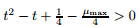Thus, is equivalent to t < t₁ or t > t₂. Besides,it can be shown that

Since 0 < ω < 2,it follows from (20) that t > . Hence,the condition (16) holds if and only if Thus,we have proved that the MSOR-like method converges if and only if the condition (19) holds. 4 Determination of optimum parameters

Following from (14) and (15),(11) is equivalent to

Therefore,we have

We let

Then,we get the following theorem.

Theorem 4.1 Let A and Q be SPD,and B be of full rank. Assume that all eigenvalues µ of Q⁻¹B^TA⁻¹B are real and positive,and ρ(M_ω ) is the spectral radius of the MSOR-like iteration matrix M_ω . Then,we get

Case 1then

Case 2then

Case 3then

where

Proof (I) If 1 − 2µ ≠ 0 or µ ≠ ,and

then

(i) If µ_min > ,then ∆₁ > 0.

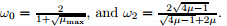
If we let

then ω₁ and ω₂ are two roots of h(ω) = 0. When ω ≤ ω₁ or ω ≥ ω₂,h(ω) ≥ 0,so ∆ ≥ 0. However,when µ_min > ,ω₁ < 0.

On the other hand,by Theorem 3.2,we have

Let ω₀ = Comparing ω₀ and ω₂,we get

when µ_max < and ω₂ < ω₀ . Letting s(µ) = ,since 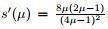,we get the following conclusions:

If µ < ,s(µ) is a monotone decreasing function. If µ > ,s(µ) is a monotone increasing function.

Therefore,if < µ_min ≤ and µ_max < 1 or µ_min > and µ_max < ,ω₂ ≤ ω₀ . By Theorem 3.2,when ω₂ < ω ≤ ω₀,∆ > 0; when 0 < ω ≤ ω₂,∆ ≤ 0.

If < µ_min < and µ_max > 1 or µ_min > and µ_max ≥ ,ω₂ > ω₀. By Theorem 3.2, when 0 < ω ≤ ω₀,∆ < 0.

(ii) If µ_min < ,then ∆₁ < 0.

When 0 < ω ≤ ω₀,h(ω) > 0 is always true,i.e.,∆ > 0 is always true. (iii) If µ = ,then ∆₁ = 0. When 0 < ω ≤ω₀,h(ω) = (1 − ) ² ω ² = ω ² > 0 is always true,i.e.,∆ > 0 is always true.

(II) If 1 − 2µ = 0 or µ = ,then h(ω) = 4ω − 4,it is easy to obtain that ∆ ≥0 if ω ≥ 1; ∆ ≤ 0 if ω < 1.

We immediately obtain

From (I) and (II) of the proof,Case (i)-Case (iii) hold,and this completes the proof.

Theorem 4.2 Let A and Q be SPD,and B be of full rank. Assume that all eigenvalues µ of Q⁻¹B^TA⁻¹B are real and positive,ρ(M_ω ) is the spectral radius of the MSOR-like iteration matrix M_ω ,ρ(M_ωb ) is the minimum of ρ(M_ω ),and ωb is the optimum relaxation factor. Then, µ_min > ,we have the following two cases. Case 1 If µ_max ≤ ,we get

Case 2 If µ_max > ,we ge

Proof From Theorem 4.1,(23) is equivalent to

That is to say,

We define

It is obviously that fω (λ) passes through the point (1,1) and gω (λ) passes through the point (0,1),respectively. For all ω,the straight line gω (λ) crosses the parabolic curve fω (λ). Similar to the analysis in ^[13],the optimal parameter ωb is the choice that guarantees that gωb (λ) is a tangent line of fωb (λ). Using the same idea,we get

Since we put (24) into (25). Then,we get = 0. Thus,∆ = 0. Since µ_min > ,it is easy to get ω_b = ω₂ = Letting = t and ω_b = we can get . Therefore,

If t < 1 or < µ < ,then ρ ² (M_ω ) is a monotonically decreasing function. If t > 1 or µ > , then ρ ² (M_ω ) is a monotonically increasing function (see Fig. 1)

(i) If ρ _µmin (M_ω ) > ρ _µmax (M_ω )(see Fig. 2),it is equivalent that

We can get

It is easy to get

Since µ_min < µ_max,we have 4µ_minµ_max ≤ (µ_min + µ_max),i.e.,µ_max ≤ .

Therefore,if µ_max ≤ ,then ρ ² (M_ωb ) = . If µ_min > ,then ρ ² (M_ωb ) = .

(ii) If ρ _µmin (M_ω ) < ρ_µmax (M_ω )(see Fig. 3),the proof of Case 2 of Theorem 4.2 is similar to that of Case 1 of Theorem 4.2. Therefore,we omit the proof of Case 2.

Theorem 4.3 Let A and Q be SPD,and B be of full rank. Assume that all eigenvalues of Q⁻¹B^TA⁻¹B are real and positive,and µ are eigenvalues of the iteration matrix of the matrix Q⁻¹B^TA⁻¹B. Let ρ(M_ω ),ρ(Ω),and ρ(M ) be the spectral radii of the MSOR-like method, MSSOR-like ^[10] method,and SOR-like ^[8] method iteration matrix,respectively. Then,we get the following result,which is a criterion for choosing between the MSOR-like,MSSOR-like,and the SOR-like methods to solve augmented systems.

Thus,the theorem is proved. 5 Numerical example

In this section,we give the example to illustrate the MSOR-like method to find the solution of the related augmented systems and compare the results of the MSOR-like method,the MSSOR-like method ^[10] ,and the SOR-like method ^[8] .

Example 1 ^[8] Consider the augmented linear system (1),in which

and

withbeing the Kronecker product symbol and h = the discretization mesh-size.

We set m = 2p² and n = p² . We choose the preconditioning matrix Q = B ^{T −1} B, =tridiag(A) for the MSOR-like,the MSSOR-like,and SOR-like methods. The stopping criterion < 10 ⁻⁶ is used in the computations,where

and is the kth iteration for each of the methods. All the computations are done on INTEL PENTIUM1.8 GHZ (256 M RAM),Windows XP system by using MATLAB 7.0. The parameters,number of iterations (IT) and CPU in seconds for convergence needed for the MSOR-like,the MSSOR-like,and the SOR-like methods are listed in Table 1 .

By observing the example,if the conditions of Theorem 4.3 are satisfied,it is not difficult to find that the MSOR-like method is superior to the MSSOR-like method and the SOR-like method. 6 Conclusions

In this paper,the MSOR-like method has been established to solve the saddle point problems, which is a simple and powerful scheme to solve (1). The convergence analysis has been given. We derive its optimal iteration parameter ω_b. From Theorem 4.3 and numerical example,it is not difficult to find that the MSOR-like method is superior to the MSSOR-like method and the SOR-like method if the conditions of Theorem 4.3 are satisfied.