 2014, Vol. 35
Article Information
- Wen-zhi ZHANG, Pei-yan HUANG. 2014.
- Coupling of high order multiplication perturbation method and reduction method for variable coefficient singular perturbation problems
- Appl. Math. Mech. -Engl. Ed., 35(1): 97-104
- http://dx.doi.org/10.1007/s10483-014-1775-x
Article History
- Received 2012-12-12;
- in final form 2013-04-09


Singular perturbation problems (SPPs) frequently occur in fluid mechanics and other branches of applied mathematics. Generally,classical numerical methods fail to achieve high accuracy because of the singularly perturbed nature. In recent years,many special methods have been undertaken for precise numerical solutions[1, 2, 3, 4, 5, 6, 7, 8, 9, 10, 11]. However,a universal way to solve SPPs is still needed at present.
The multiplication perturbation method[12] proposed by Tan and Zhong can be considered as a first-order multiplication perturbation method for time-varying systems. Fu et al.[13] further proposed a high order multiplication perturbation method (HOMPM),which enabled the precise integration method (PIM) for time-varying ordinary differential equations (ODEs) to reach the same accuracy as that of the PIM proposed by Zhong and Williams[14] for constant coefficient problems.
In this paper,a coupling technique of the HOMPM and the reduction method is developed to provide an efficient method for the variable coefficient singularly perturbed two-point boundary value problems (TPBVPs) with one boundary layer. The present method can have both the improved accuracy with increased orders of the HOMPMand the high efficiency of the reduction method. Thus,it has a bright application future.
2 Method descriptionConsider the following variable coefficient SPP:
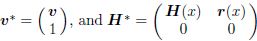
where ε is a small positive parameter (0<ε <<1),and α and β are known constants. We transform Eq. (1) into a system of first-order ODEs by introducing p(x) = y′(x). Thus, where Conducting dimensional expanding[15] with Eq. (3),we have where


Thus,in the following,we only need to solve the homogeneous equation (4).
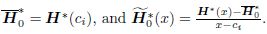
First,divide the interval [0, 1] with τ = 1/m. Let xi = iτ (i = 0,1,· · · ,m) and ci= xi + τ/2 .Then,discompose H*(x) as
where
Let
Substituting Eq. (6) into Eq. (3),we obtain where


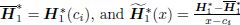
Then,discompose H1*(x) as
where
Furthermore,let
in which N is the final times of perturbation.
Obviously,
in which
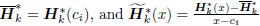
Similarly,Hk*(x) is discomposed as
where
Ignoring the high order item  ,we obtain


Define
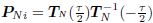
We have Let x = xi in Eq. (15). We get where


Let x = xi+1 in Eq. (15). Then,
where
 is the transfer matrix.
Equation (17) cannot be solved directly by the HOMPM. Thus,we use an efficient reduction method to solve it. Let m = 2M + 1,and substitute Eq. (2) into Eq. (17). Then,
where We add the (2k−1 + 1)th equation multiplied by −C(k−1) L to the first equation,and add the (m−2k−1)th equation multiplied by −(A(k−1) RB +A(k−1) RS ) to the last one. At the same time,add each (2kj+1−2k−1)th equation multiplied by −( A(k−1) (2kj)B + A(k−1) (2kj)S) and the (2kj+1+2k−1)th equation multiplied by −C(k−1) 2kj to the (2kj + 1)th equation (j = 1,2,· · · ,2M−k − 1,k = 1,2,· · · ,M),which gives where in which


 After M times of iterations,the system becomes
in which
After M times of iterations,the system becomes
in which

The solution of Eq. (20) is After u1(M) is given,all the required solutions of Eq. (1) can be worked out through the reversed reduction process.
3 Numerical examplesExample 1 Consider the SPP

It has one boundary layer at x = 1,and the exact solution is y(x) = . To solve this
problem,we let N = 0 and M = 0 for ε = 10−2 and ε = 10−3 (when N = 0,the method of this
paper degrades into the method in Ref. [16]). After y′(1) is given,redivide the mesh and use
v*(xi) = P−1
N(i+1)v*(xi+1) to get the solutions from right to left with τ = 0.01. The numerical
solutions given by the present method are displayed in Table 1 together with Chawla’s and
Andargie’s solutions.
. To solve this
problem,we let N = 0 and M = 0 for ε = 10−2 and ε = 10−3 (when N = 0,the method of this
paper degrades into the method in Ref. [16]). After y′(1) is given,redivide the mesh and use
v*(xi) = P−1
N(i+1)v*(xi+1) to get the solutions from right to left with τ = 0.01. The numerical
solutions given by the present method are displayed in Table 1 together with Chawla’s and
Andargie’s solutions.
From Table 1 ,we can see that the present solutions are exactly the same as the exact solu- tions. Obviously,the present method is much more precise than the other numerical methods. Therefore,the present method has an outstanding advantage in solving constant coefficient SPPs.

To show the efficiency of the present method,we compare its computation time with that of Ref. [4] (see Table 2 ).

Example 2 Consider this variable coefficient SPP
It has one boundary layer at x = 0,and the analytical solution is [17] First,let N = 2 for ε = 10−2 with M = 3 and ε = 10−3 with M = 6. Remesh the grid with τ = 0.01 after y′(0) is obtained to compute the required solutions in the desired points. To show how precise the present method is,we compare the numerical solutions of the present method with those of Refs. [4] and [1] (see Table 3).


It can be easily noticed from Table 3 that in the boundary layer,the solutions of the present method are obviously much better than those of Refs. [4] and [1].
The computation time of the present method is also compared with that of Ref. [1] (see Table 4 ).

It can be noticed from Table 4 that the computation time of the present method is a bit longer than that of Ref. [1],which is partly due to the redivision of grids for computation after y′(0) is worked out.
4 ConclusionsWe present a coupling technique of the HOMPM and the reduction method for variable coefficient singularly perturbed TPBVPs with one boundary layer. This method combines the advantages of the HOMPM and the reduction method. Thus,it is highly accurate and efficient. The present method extends the application of the PIM to the solution for variable coefficient SPPs and also provides a new way to solve other variable coefficient TPBVPs.
| [1] | Chawla, M. M. A fourth-order tridiagonal finite difference method for general non-linear two-point boundary value problems with mixed boundary conditions. Journal of the Institute of Mathematics and Its Application, 21, 83–93 (1978) |
| [2] | Kadalbajoo, M. K. and Patidar, K. C. A survey of numerical techniques for solving singularly perturbed ordinary differential equations. Applied Mathematics and Computation, 130, 457–510 (2002) |
| [3] | Vigo-Aguiar, J. and Natesan, S. An efficient numerical method for singular perturbation pro- blems. Journal of Computational and Applied Mathematics, 192, 132–141 (2006) |
| [4] | Andargie, A. and Reddy, Y. N. Fitted fourth-order tridiagonal finite difference method for singular perturbation problems. Applied Mathematics and Computation, 192, 90–100 (2007) |
| [5] | Chakravarthy, P. P., Phaneendra, K., and Reddy, Y. N. A seventh-order numerical method for singular perturbation problems. Applied Mathematics and Computation, 186, 860–871 (2007) |
| [6] | Herceg, D. and Herceg, D. On a fourth-order finite-difference method for singularly perturbed boundary value problems. Applied Mathematics and Computation, 203, 828–837 (2008) |
| [7] | Evrenosoglu, M. and Somali, S. Least squares methods for solving singularly perturbed two-point boundary value problems using B′ezier control points. Applied Mathematics Letters, 21, 1029–1032 (2008) |
| [8] | Habib, H. M. and El-Zahar, E. R. Variable step size initial value algorithm for singular pertu- rbation problems using locally exact integration. Applied Mathematics and Computation, 200, 330–340 (2008) |
| [9] | Lubuma, J. M. S. and Patidar, K. C. Toward the implementation of the singular function method for singular perturbation problems. Applied Mathematics and Computation, 209, 68–74 (2009) |
| [10] | Kumar, M. and Mittal, P. A. Methods for solving singular perturbation problems arising in science and engineering. Mathematical and Computer Modelling, 54, 556–575 (2011) |
| [11] | Goh, J., Majid, A. A., and Ismail, A. I. M. A quartic B-spline for second-order singular boundary value problems. Computers and Mathematics with Applications, 64, 115–120 (2012) |
| [12] | Tan, S. J. and Zhong,W. X. Numerical solution of differential Riccati equation with variable coeffi- cients via symplectic conservative perturbation method (in Chinese). Journal of Dalian University of Technology, 46(S1), S7–S13 (2006) |
| [13] | Fu, M. H., Lan, L. H., Lu, K. L., and Zhang, W. Z. The high order multiplication perturbation method for time-varying dynamic system (in Chinese). Scientia Sinica-Physica, Mechanica and Astronomica, 42, 185–191 (2012) |
| [14] | Zhong, W. X. and Williams, F. W. A precise time step integration method. Proceedings of the Institute of Mechanical Engineers Part C, Journal of Mechanical Engineering Science, 208(C6), 427–430 (1994) |
| [15] | Gu, Y. X., Chen, B. S., Zhang, H. W., and Guan, Z. Q. Precise time integration method with dimensional expanding for structural dynamic equations. AIAA Journal, 39(12), 2394–2399 (2001) |
| [16] | Fu, M. H., Cheung, M. C., and Sheshenin, S. V. Precise integration method for solving singular perturbation problems. Applied Mathematics and Mechanics (English Edition), 31(11), 1463–1472 (2010)DOI 10.1007/s10483-010-1376-x |
| [17] | Nayfeh, A. H. Perturbation Methods, Wiley, New York (1979) |