 2014, Vol. 35
Shanghai University
Article Information
- Zuo-jin ZHU, Jian-lei NIU, Ying-lin LI. 2014.
- Swirling-strength based large eddy simulation of turbulent flow around single square cylinder at low Reynolds numbers
- Appl. Math. Mech. -Engl. Ed., 35(8): 959-978
- http://dx.doi.org/10.1007/s10483-014-1847-7
Article History
- Received Jun. 25, 2013
- Revised Sept. 16, 2013


2. Faculty of Construction and Environment, The Hong Kong Polytechnic University, Hung Hom, Kowloon, Hong Kong, P. R. China
Incompressible turbulent flows around a single square cylinder (SC) are basically taken as a crucial academic problem in the society of applied mathematics and mechanics,since in fact there exist long-time interests of deeply perceiving the characteristics and properties of the turbulent SC flows.A brief literature review of the works done before the year 1990 was given previously[1],which was prepared for the project of larger mechanics problem in ocean engineering financially supported by national science foundation of china (NSFC) in the latter of 1980s.Here,we trace the research history from two lines before presenting the objective of this paper. 1.1 Experiments
The earlier encompassment was reported in 1966 by Vickery[2],where the influence of incom- ing stream turbulence intensity on the lift and drag on a long cylinder of square cross-section was explored.Similarly,some studies were done to seek the turbulence effect on drag of rectan- gular cylinders[3, 4, 5, 6].Some measurements of SC wake were carried out by Okajima[3] and Davis et al.[7].The flapping shear layer formed by flow separation from the forward corner of an SC was studied experimentally by Lyn and Rodi[8].By virtue of one-component laser-Doppler velocimetry,they also investigated the associated recirculation region on the sidewall formed in flow separation from the forward corner of an SC.It was suggested that the recirculation effect can be a possible explanation for some flow properties.
On the other hand,Gu and Sun[9] carried out wind tunnel tests to measure the interference between two circular cylinders (CC) in staggered arrangement at high subcritical Reynolds numbers (i.e.,2.2 × 105 and 3.3 × 10⁵),and found three main flow patterns.They also mea- sured the flows around three parallel CC in equilateral-triangular arrangements by wind tunnel tests[10].By measuring pressure distributions on three CC at Reynolds number 5.5 × 10⁴ and visualizing flow regimes at Reynolds number 1.4×10⁴,when the spacing ratio is over the range 1.7≤6 N/d 6≤2.2,where N and d are respectively the distance between the centers of adjacent cylinders and the cylinder diameter,there are three basic interference types: interference of proximity,shear layer reattachment,and wake.As the incident angle varies from zero to 60°, these flow patterns can be subdivided further.
Recently,using dye- and laser-induced fluorescence visualizations,the spanwise and stream- wise vortex structures were captured by Luo et al.[11].It was found that the critical Reynolds numbers were in the range from 160 to 200,at which mode transition from the mode A to B occurs.For the flow pattern mode A or B,the spanwise wavelengths are slightly different from that observed in CC flow.Highlighting the effect of incoming flow turbulence,after particle imaging velocimetry (PIV) measurements,So et al.[12] found that the incoming flow turbulence increases the vortex shedding frequency in the post-lock-in region but does not change the system natural frequency.The so-called lock-in point is the point at which the frequency of vortex-shedding frequency coincides with the system natural frequency.
For wake flows,many concluding remarks can be found in recent literatures.For instance, to study the vortical structures and the interactions in the turbulent wakes of three side-by-side circular CC,Zhou[13] measured the turbulent wake using various techniques,including PIV, hot-wire anemometry,laser Doppler anemometry,and laser-illuminated flow visualization.The cylinder centre-to-centre spacing T/d is arranged to be 1.5,at which both wide and narrow wakes exist.It can be observed that the base pressures of the upper and lower cylinders are identical but smaller than that of the central cylinder.Consequently,the gap flows between cylinders are deflected towards the upper and lower cylinders,respectively,forming one wide wake behind the central cylinder and one narrow wake on each side of the wide wake.It was indicated that while the vortical structures in the narrow wakes may be generated from the shear layer separation from the upper or lower cylinder,those in the wide wake may originate from the shear layer instability.
For the near wake around a finite-length SC,with one end mounted on a flat plate and the other free,an experimental study was carried out by Wang and Zhou[14].The cylinder aspect ratio,or height-to-width ratio H/d ranges from 3 to 7.The Reynolds number based on d and the free-stream velocity is 9 300.Using the hot-wire anemometry,laser Doppler anemometry, and PIV,measurements were carried out mainly in a closed-loop low-speed wind tunnel.It was reported that the instantaneous flow structure around the cylinder is arch-type regardless of H/d,consisting of two spanwise vortical “legs”,one on each side of the cylinder,and their connection or “bridge” is near the free end.
For Reynolds number in the range of (2 500,6.0 × 104),Alam et al.[15] measured the CC wake flows using two tripwires attached at azimuthal angle alpha = ±10° to 70° measured from the forward stagnation point.Based on the measurements and those in literature,five flow regimes (A - E) are classified.In particular,it was proposed that the bi-stable phenomenon (regime D) has its possible connection to the mechanism of well reported rain-wind-induced cable vibration.
A systematic experimental study of the flow past two side-by-side square cylinders was carried out by Alam et al.[16].Using different techniques,including hot wires,load cell,PIV and laser-induced fluorescence flow visualization,the flow experiments were performed at Re = 4.7 × 10⁴ and a changeable cylinder centre-to-centre spacing ratio (T/d) ranged from 1.02 to 6.00.Based on the flow structure and the Strouhal number (St),four distinct flow regimes and their corresponding T/d ranges are identified.The results also unveil a crucial role played by the gap flow and its passage geometry in contributing to the differences observed.
In addition to the significant insights from experiments,the onset of instability in the flow around an SC with linear stability analysis was studied by Kelkar and Patankar[17].It was reported that the critical Reynolds number is inferred from the variation of the rate of growth of the perturbations with the Reynolds number.For unsteady flow at a Reynolds number above the critical value,the calculated Strouhal number is very close to its experimentally observed value.Furthermore,a stability analysis revealed that there is a critical Reynolds number beyond which the SC wake flow turns to three dimensional regime,as reported by Robichaux et al.[18]. On the other hand,for CC wake flow,the corresponding vortex dynamics has been reviewed by Williamson[19].Both extrinsic and intrinsic features are described in detail. 1.2 Simulations
Using different turbulence models,numerical simulations of vortex shedding past a free- standing SC at Re = 2.2 × 10⁴ were done by Bosch and Rodi[20].Using wall functions,the standard k - ε model was compared with a modification suggested by Kato and Launder[21]. It was shown that the main quantities of engineering interest can be predicted reasonably well with k -ε type models.The application of the KatoõLaunder modification can bring a major improvement.
A direct numerical simulation (DNS) of three-dimensional flow around an SC at Reynolds numbers ranged from 150 to 500 was carried out by Sohankar et al.[22].In the DNS,the grid is non-staggered,and the pressure Poisson equation is solved by a multi-grid approach,implying that some numerical disturbances should have been unexpectedly introduced into the DNS software,for which,some explanations can be found in the previous work[23, 24].
Similarly,to predict the appearance of three-dimensional phenomena in the flow past an SC numerically,the DNS results for the scenarios of Reynolds numbers from 125 to 500 were reported by Saha et al.[25].It was found that the values of the Strouhal number and the time-averaged drag-coefficient are closely associated with each other and can reflect the spatial structure of the wake.It can be noted that their results are based on the MAC algorithm of Harlow and Welch[26].Noticeably,in the numerical approximation,both the convective and diffusive terms are dealt with the central difference scheme.
To understand air pollutant dispersion among high-density,high-rise buildings,Niu and Zhu[27] reported the numerical results of three-dimensional flows around two identical square cylinders in staggered arrangements at Reynolds number 250 and zero incident angle,when the angle between the incoming velocity vector and the line connecting the centers of the cylinders is 45°.
Niu et al.[28] reported the numerical results of convective heat transfer from two identical square cylinders (TISC) arranged at close proximity in a uniform cross air-flow at Re=250.It can be found that depending on the TISC arrangement,a bifurcation sometimes occurs,with the bifurcated lower Strouhal number value corresponding to the shedding from the outer shear layer,and the higher one corresponding to the shedding from the inner shear layer.
The numerical scheme in the previous studies[22, 25, 27] can be further improved by using a 4th order upwind scheme to deal with the nonlinear convective terms in the governing equations. Actually,in a staggered grid system,numerical approximation by interpolation should adhere to the law of Taylor expansion,otherwise,the discrepancy in numerical solution can occur,because in numerical scheme design the implicitly-introduced artificial-viscosity due to truncation error is comparatively high.
In general,for turbulent flow simulations,three strategies: the phenomenological models, the DNS,and the large eddy simulations (LES) are widely used.The first strategy was reviewed by Hanjalic[29].It was based on Reynolds averaging,but the lacking of universal property for the model coefficients implies that these coefficients examined in some benchmark situations might be unsuitable to other relatively complicated engineering problems.
The DNS,as reported in Refs.[30, 31, 32],in the traditional meaning,should use extremely fine grids so that the total spatial grid numbers should be as large as Re2.25,where Re is the Reynolds number.This indicates that super computers must be used in DNS of fully developed turbulent flows.
The LES,as reported in Refs.[33, 34],uses the grid-filtering to explicitly simulate the large motion,while the small eddy effect on the large eddy motion should be modeled.The LES works reported previously[35, 36, 37, 38, 39, 40, 41, 42] indicate that this is an appropriate strategy for predicting turbulent flows.
For the LES,a series of sub-grid scale (SGS) models were developed[35, 43, 44, 45, 46, 47, 48],among which are the earlier SGS model of Smagorinsky[35],the dynamic SGS model given by Germano et al.[43],a modification of dynamic SGS model[44],the SGS model based on the Kolmogorov equation for resolved turbulence[45, 46],the Vreman model based on algebraic theory,and the recent SGS model based on dynamic estimation of Lagrangian time scale developed by Verma and Mahesh[48].However,it should be noted that the SGS models reported so far have not ascertained under what flow conditions the LES can lapse into the DNS.
It should be mentioned that even in LES the unclosed stresses are usually modeled by SGS-viscosity models,alternatively,to smooth the dynamics of the Navier-Stokes equations, another way is to directly modify the non-linear convective terms[49].Thus,models based on these regulations occur[50, 51, 52, 53, 54, 55].
Turbulent flow is intermittent in time and space,indicating that at a local point the flow may be swirling or non-swirling,depending on if the swirling strength value is non-zero,or zero. The SGS model described in this paper can extent reflect this flow property.The results of the LES are compared with existing experimental data. 1.3 Objective
This paper presents the swirling-strength based on the LES results of the incompressible zero-incident flows around a single SC at low Reynolds numbers in the range from 103 to 104. The objective is to explore the SC flow characteristics,primarily related to three aspects: (i) the Reynolds number dependence,(ii) the distribution of (t-z) averaged vorticity component and sub-grid viscosity ratio,and (iii) the distribution of the (t-z) averaged Kolmogorovmicro-scale. 2 Governing equations
At higher Reynolds numbers,turbulent effect is significant,so the SGS effect on large scale motions should be carefully considered.In previous LES works[36, 37, 38, 39, 40, 41, 42],sub-grid stress is usually assumed to be the product of sub-grid viscosity and filtered strain rate,which is just an analogy of the constitutive relationship for laminar Newtonian fluid flows.This indicates that these SGS models have not satisfactorily ascertained at what Reynolds number they are applicable, because the sub-grid viscosity still exists,even when the flow is switched to a laminar regime and the swirl strength is generally zero.
In the earlier work of Smagorinsky[35],the sub-grid viscosity is assumed to be proportional to the modular of local strain rate of filtered velocity field.But unfortunately,using the three- dimensional velocity fields based on flow instability analysis[56],numerical tests revealed that the peak values of the modular of strain rate occurs at regions without swirling.To overcome this ambiguity,considering that turbulent flows have coherent structures and strong intermittency, here we propose a relatively fresh SGS model,where the sub-grid viscosity is supposed to be proportional to the FSI and local swirling strength,
Here,Cμ (= 0.09) is an artificially-defined constant,λci is the swirling strength of filtered velocity gradient ∇u,the FSI,fI,is the ratio of swirling strength λci to the magnitude of the complex eigenvalue λ (= λcr + iλci) of ∇u,i.e., where δ is the length scale,defined by harmonic-average of grid intervals, where δi denotes the grid interval in the xi direction.If the filtered velocity gradient ∇u is denoted by its eigenvalue λ must satisfy the characteristic equation where with |A| representing the determinant of A.If the turbulent flow is not affected by the Coriolis force due to coordinate rotation,at a local point if the roots of (5) are real,and the swirling strength equals zero,it indicates that the vortices certainly have not arrived at the point, implying that the local flow regime is temporally laminar.On the other hand,when the local flow is in a turbulent regime,it indicates that there are vortices at the local point,suggesting that the roots must have two conjugate complex eigenvalues denoted by λcr ± iλci,here,i (=


 ) is the unit of imaginary number.The iso-surfaces of swirling strength were used to
illustrate vortices in turbulent flows previously[57, 58, 59].
) is the unit of imaginary number.The iso-surfaces of swirling strength were used to
illustrate vortices in turbulent flows previously[57, 58, 59].Because the sub-grid viscosity νs has a factor fI,the decaying factor of the length scale (1-exp(-y+/25)) near the wall as used in previous study[36] is abolished in the present study, where y+ = yuτ/ν,y denotes the normal distance to the wall,with uτ denoting the mean friction velocity and ν representing the kinematic viscosity of fluid.
Since the swirling strength can occur in laminar flow regime when there is the effect of Cori- olis force due to coordinate rotation,in order to see the peculiarity of the present SGS model,a comparison of the present model with that of Vreman[47] is therefore given in Figs.1(a)-1(b), where two top-views of the contours of sub-grid viscosity are illustrated.It can be seen that the sub-grid viscosity based on the present model is zero if the flow is non-swirling,while sub-grid viscosity based on the Vreman model does not hold this peculiarity.
 |
| Fig. 1.Comparison of sub-grid model with previous one proposed by Vreman[47](note that sub-grid viscosity has unit of W0d0 as seen in Appendix A,contours in part (a) are labeled by values from 0.000 4 to 0.001 6 with increment of 0.000 3,while contours in part (b) are labeled by values from 0.000 4 to 0.012 with increment of 0.002 9) |
Consider the turbulent SC flows in a Cartesian coordinate system,as schematically shown in Fig. 2,in which x is the horizontal coordinate,while y and z denote the vertical and spanwise directions.The origin (O) is allocated at the left-bottom corner of the SC.The spanwise coordinate is given merely by the symbol z.Let the fluid kinematic viscosity be ν,for the incoming flow velocity uin,the Reynolds number of the SC flow can be defined by Re = uind/ν.
 |
| Fig. 2.Schematic of zero-incident turbulent flow around single SC |
We select u0 = uin and the SC cross-sectional side length d as the velocity and length scales,hence the time and pressure scales should be t0 = d/u0 and ρu0 2 .Here,ρ is the fluid density.The dimensionless governing equations for the incompressible SC flows can be written as follows:
For simplicity of presentation,here we have omitted the over bar for filtering of variables.The normalized total viscosity γ1 can be represented by R denotes a force depending on viscosity gradient,


The solutions of (7) and (8) are sought under appropriate boundary and initial conditions. For the boundary conditions (BC) on the SC walls,non-slip BC is used,which implies
while for the BC at the outlet,similar to the treatment published elsewhere[22, 25],we use the Orlanski[60] type In the normalized form,we choose uc = 1.At the inlet section,we choose However,on the lower and upper side boundaries of the computational domain,we use The initial condition is given by The periodical condition is used on the spanwise boundaries,which can be simply expressed as where B is the spanwise (z) length of the SC (see Fig. 2). 3 Numerical method 3.1 Solution procedure


The governing equations (7)-(8) of the SC flow problem were discretized by a finite difference method in a staggered grid system,where the convective terms were treated using the 4th order upwind scheme[61].It can be noted that by making some proper changes,the existing numerical methods[24, 26, 62, 63, 64, 65, 66] should also be applicable.
The solution procedure is based on the accurate projection algorithm PmIII developed by Brown et al.[67].The detailed steps of the procedure were described elsewhere[68].Now just a brief description is described below.
Let the intermediate velocity vector,the pressure potential,and the time level be u,φ,and n,respectively.Define H = (u · ∇)u - R,then let
We can calculate u by and calculate pressure p by where the pressure potential φ must satisfy the Poisson equation and the terms at the level of (n + 1/2) are calculated explicitly using a second order Euler prediction-correction scheme in temporal.As mentioned above,the nonlinear convective terms in the governing equations are spatially discretized by the 4th upwind finite difference scheme given in Ref.[61],with the viscous diffusion terms by the second-order central difference scheme.


The pressure potential Poisson’s equation is solved by the approximate factorization one (AF1) method[69] at first,and then by the stabilized bi-conjugate gradientmethod (Bi-CGSTAB) given by van der Vorst[70] to improve the solution accuracy.In the AF1 application,for the SC wake flow simulation,the numerical experience reported elsewhere[1] is useful for the nu- merical stability of pressure potential iteration.The criterion for pressure potential iteration was chosen so that the relative error defined previously[71] should be less than 3 × 10⁻⁸.The implicit second-order Crank-Nicolson for the right-hand side diffusion terms are used in spatial discretization. 3.2 Scheme improvement
Considering its intrinsic potential in numerical simulation[24],the staggered grid system is used.we have therefore arranged uijk,vijk,and wijk at the points P1(x-1/2+i,yj,zk), P2(xi,y-1/2+j,zk),and P3(xi,yj ,z-1/2+k),respectively,with pressure potential φijk set at point P(xi,yj,zk).Based on this stagger arrangement,the non-linear convective terms in the momentum equations are spatially discretized with a 4th order upwind scheme,in which those terms at the level o(ε4) are neglected.To briefly describe this scheme,we just give an expression for uux in the u-momentum equation.Adhering to the upwind idea,omitting the subscripts of j and k,for uux at P1,when u(x-1/2+i,yj,zk) = ui > 0,we have
otherwise, The scheme coefficients can be obtained by the Taylor expansion,for ui > 0, where δ1 = +x-1/2+i - x-1/2+i-1,δ2 = +x-1/2+i - x-1/2+i-2.On the other hand,when ui≤6 0,we have where δ1 = -x-1/2+i+x-1/2+i+1,δ2 = -x-1/2+i+x-1/2+i+2.For vuy and wuz,i.e.,the cross-convective terms in the u-momentum equation,some descriptions were reported elsewhere[61]. Similar numerical treatments can be encompassed for the v- and w-momentum equations.It is necessary to mention that to comparative-rigorously adhere to the upwind concept,the value of ux(3) must be yielded at x-1/2+i-1/2 for ui > 0,or at x-1/2+i+1/2 for ui < 0.Correspondingly, some Taylor-expansion-based modification for the scheme coefficients (A,B,C,and D) is required. In particular,for numerical treatment of the divergence of intermediate velocity vector ∇·u and the ∇2φ at the time level n,the influences of heterogeneous stagger grid (i.e.,φi is arranged between ui and ui+1) are taken into account to improve the accuracy of spatial discretization. 4 Results and discussion


In terms of the numerical method described above,the LES of the single SC flows as shown schematically in Fig. 2 was encompassed using an Inter-Cored personal computer with a memory 3.2 Gb and a CPU frequency 3.30 GHz.Correspondingly,the geometrical parameters for computational domain were given in Table 1.Each case requires a CPU time of about 68 hours.Classified by Re3 = Re/103,6 cases were studied,as shown in Table 2.For each case, the spanwise length of the SC (B) is set as 11.

 |
The grid in z -direction is uniform,with grid number Nk=41.While the grids in x- and y- directions are non-uniform,the grid-numbers are 191 and 145,respectively.The grid-partition uses a geometrical-series algorithm.The grid,in principle,should be denser near the SC walls. That means the grids near SC corners must be denser.The assignment of grids on the SC section walls has used two key parameters named as the amplifying-factor(1/0.88),the series termination number (14).The total number of vertical grid-line passing through the SC cross- sectional side is 34,as indicated in the range of x ∈ [0, 1] in Fig. 3(a).
 |
| Fig. 3.x - y grid distributions near single SC (note that δxi = xi - xi-1,Δyj = (yj+1 - yj-1)/2, and side length of SC is unity) |
The grid heterogeneity near the SC can be seen in Figs.3(a) and 3(b).In the bottom and top sides of the SC,the y-grid is assigned with an amplifying-factor 1/0.85 and a series- termination number 17.While for x-grid assignment,the relevant values are 1/0.828 and 17 for the region upwind the SC,but 1/0.935 and 47 for the region downstream the SC.Using the geometrical-series algorithm for grid partition,it seen that the finest grid distance to each SC wall is 4.165 × 10⁻³.Such a grid arrangement leads to a time step Δt = 2.125 × 10⁻³,which is smaller than those reported previously[22, 25, 27].
Just in the xy-plane,to show the distribution of Kolmogorov micro-scales,which are ob- tained by time-spanwise (t-z) averaging,we use a subscript “m” to represent (t-z) averaged variables,and a superscript (′) to represent the root mean square values (RMS) of the variables. Especially,the subscript “m” was omitted for (t - z) average lift (CL) and drag (CD),just for the convenience of representation.For Re ∈ [103,104],the vortex motion can result in relatively complicated flow patterns,which should be explored carefully and appropriately.It is noted for the 6 cases,the grid arrangement and the time step are unchanged.In post-processing of the LES output data,to remove the effect of initial condition,merely the data in the time period of t ∈ [68, 170] are used.The aspects of flow induced forces,and flow patterns are reported and discussed in the following subsections. 4.1 Flow characteristics
For turbulent SC flows,the characteristics can be recognized by observing the CD and CL coefficients,their mean and RMS values.The RMS values should be corresponding to the time averaging for the temporal data train obtained from the CD and CL coefficients based on z- average.Because the SC flows have fixed vortex separation points,the vortex shedding should be different from that in a CC flows.
To illustrate the Reynolds number dependence,the (t - z) averaged CL,CD,(νsr)pm,their relevant RMS values denoted by CL′,CD′ and (νsr)′ p,and the Strouhal number are given in Table 2,Figs.4(a)-4(b),and Figs.5(a)-5(b).As shown in the third column of Table 2,for Re3 = Re/103 ∈ [2.5,10],the mean CD is about 1.825 (±0.052),with the maximum of relative deviation being 2.83%.This means that over the range of Re3 ∈ [2.5,10],the drag coefficient is almost certainly Reynolds-number independent.For Re3 ∈ [1,2.5],also given in the third column of Table 2,it can be seen that the present λci-based LES indicates that with the increase of Reynolds number,the mean CD increases gradually from 1.605 to 1.775.Furthermore,as seen in the second column of Table 2,the mean CL is approximately zero.Also,this Reynolds- number dependence of mean CD and CL,can be observed in Fig. 4(a).
 |
| Fig. 4.Reynolds number dependence of mean CL and CD,RMS of CL and CD,and time-averaged viscosity ratio (νsr)pm as well as its relevant RMS (νsr)′ p (note that (νsr)pm is calculated merely by time-averaging for peak value of νsr in computational domain) |
It should be mentioned that for Re = 500 (Re3 = 0.5),the mean CD is 1.84,or 2.17 as respectively reported in the DNS[22, 25].This suggests even if the numerical results are based on DNS,the difference still exists due to the different solution procedure.On the other hand,the earlier measurements[4, 5, 6] indicated the mean drag coefficient CD is around 2.0.As reported previously[1],for turbulent flow around a single SC,the mean CD value depends on the turbulence intensity of incoming flow,an increase of the intensity can cause a decease of the mean CD.
The Re dependence of relevant RMS values denoted by CL′,CD′,and (νsr)′ p can be seen from the 5th,6th,and 7th columns of Table 2.Different from the work of Bosch and Rodi[20], these values are obtained on the basis of the current three-dimensional (3D) LES,where the sub-grid viscosity is calculated in terms of (1).Corresponding to the values given by the 5th and 6th columns of Table 2,the CL′ and CD′ are plotted as functions of Re3,as seen in Fig. 4(b). Coarsely seen,in the low Re number range of Re3 ∈ [1, 10],the CL′ is approximately 0.2,with CD′ having a value around 0.1.
It is noted that the peak value of viscosity ratio (νsr) is sought in the whole 3D computational domain.Because the turbulent SC flow is intrinsically dynamic,the peak value point must be varied temporally.The mean peak value denoted by (νsr)pm is merely based on t-average.From Fig. 4(c),it can be seen that the mean peak value of viscosity ratio (νsr)pm and its RMS value exhibit growing trend with Reynolds number,but the growing rate for (νsr)pm is larger.For instance,at Re3 = 10,the (νsr)pm value is 17.16 with its RMS value equal to 3.673,as can be seen from the 7th line of Table 2.
Crucially,the Strouhal number has an evident independence of Reynolds number,as seen
in 8th column of Table 2.For Re3 ∈ [1, 10],St is about 0.112 8 with a relative deviation less
than 4.5%,which can also be seen clearly from Figs.5(a)-5(d),in which the power spectra
at Re3 = 1,2,2.5,and 10 for parts 5(a)-5(d) are obtained by discrete Hilbert transform as
done previously[72].This Strouhal number is very close to the St number 0.124 for the case of
Re = 2.2 × 10⁴ (or Re3 = 22) as predicted by Bosch and Rodi[20],when the two-dimensional
flow calculation was based on the two-layer (TL) approach with Standard k -ε equation when
the inlet viscosity ratio (rμ = νt/ν) was set as 100.Note νt is the eddy viscosity which depends
on kinetic energy k and its dissipation rate ε.As reported[20],the Strouhal number measured
by Bearman and Trueman[4] is 0.123 for the SC flow at Re ≈ 5 × 10⁴ (or Re3 ≈ 50) when
the inlet flow turbulence level T u (=  was less than 1.2%.For Re = 500,the previous
DNS[22, 25] indicated that the Strouhal number value is 0.122,or 0.116 respectively,which shows
that the present LES has predicted the Strouhal number agreed quite well with that on the
basis of DNS of the single SC flow at Re = 500.
was less than 1.2%.For Re = 500,the previous
DNS[22, 25] indicated that the Strouhal number value is 0.122,or 0.116 respectively,which shows
that the present LES has predicted the Strouhal number agreed quite well with that on the
basis of DNS of the single SC flow at Re = 500.
 |
| Fig. 5.Power spectra of evolutions of CD and CL |
The relevant evolutions of lift and drag at Re3 = 2.5 can be seen in Figs.6(a)-6(b),from which a visual comparison with c-DNS can be made.Obviously,for Re3 = 2.5,the SC flow is turbulent,the use of λci-based sub-grid viscosity model has not brought large discrepancies of the evolution curves of z-averaged lift and drag coefficients.
 |
| Fig. 6.Comparison of LES and c-DNS with respect to evolutions of lift and drag at Re3 = 2.5 |
This comparison again provides numerical-solution evidence for the Chinese Society of Me- chanics to believe that the nonstandard analysis theory of turbulence[73, 74, 75],is to some extent correct,and can be applied to get a higher computational efficiency as reported elsewhere[61, 68]. This nonstandard analysis theory allows the use of c-DNS to obtain relatively accurate results, unnecessary to follow the DNS grid number requirement: be at the level of Re2.25.
The properties of the peak value of viscosity ratio can be ascertained by reading in the evolution given by Fig. 7,from which we can see that both the mean peak value of viscosity ratio (νsr)pm and its RMS value have growing tendency,as seen directly in Fig. 4(c).The values of (νsr)pm given by Fig. 7 implies that there exists a consistency when those given by Table 2 were compared just for the cases of Re3 = 2.5 and 10.
 |
| Fig. 7.Comparison of peak value of viscosity ratio ((νsr)p ≡ (νs/ν)peak) with respect to corresponding evolutions at Re3 = 2.5 and 10 |
This consistency can also be evidently seen from Figs.8(a)-8(b).As given by Table 2,it is seen that at Re3 = 2.5,CD′ ≈ 0.1; while at Re3 = 10,CD′ = 0.128 8.In Fig. 8(b),it easily seen that the oscillation of CD in the period of t ∈ (140,170) does have a larger fluctuation magnitude.
 |
| Fig. 8.Evolutions of lift and drag coefficients at Re3=2.5 and 10 |
The flow patterns vary temporally and spatially[76, 77, 78].The illustration of the turbulent flow patterns is useful to deepen the understanding of the zero-incident incompressible flows around a single SC at low Reynolds numbers located in the range Re ∈ [103,104].
When t = 170,the contours of vorticity component ω1 at x = 3,6,9,and 12 for Re3 = 2.5 are shown by Figs.9(a)-9(d),i.e.,the top-layer,with the relevant ω1 contours for Re3 = 10 given by Figs.9(e)-9(h),i.e.,the bottom-layer.A comparison between the layers of Fig. 9 reveals that the secondary flow pattern are Re dependent.While a comparison between parts 9(a)-9(d) in the top-layer or parts 9(e)-9(h) in the bottom-layer indicates that the secondary flow pattern is x-dependent.
 |
| Fig. 9.Contours of streamwise vorticity component (ω1) at t = 170,and four x-locations (i.e.,x=3,6,9,and 12) for Re3 = 2.5 and Re3=10 (note that contours are labeled by -0.3,-0.2,-0.1, 0,0.1,0.2,and -0.3) |
There is an intrinsic correlation between the secondary flows (see Fig. 9) and the main stream flow patterns shown by contours of ω3 as seen in Figs.10(a)-10(b).Note that the calculation of flow vorticity components has utilized the advantage of staggered grid arrangement.For instance,the (ω3)ijk stored at the point (x-1/2+i,y-1/2+j ,zk) can be predicted more conve-niently.
 |
| Fig. 10.Contours of spanwise vorticity component (ω3) at t = 170,and z = 5.5 for Re3 = 2.5,and Re3=10 (note that contours of ω3 are labeled by -2,-1,-0.5,0,0.5,1,and 2) |
Even though at the peak value of viscosity ratio can change its spatial position as a result of large eddy motion in the 3D computation domain,exploring where the peak value could appear should be useful for understanding the characteristics of turbulent SC flows at low Reynolds numbers.Therefore,the (t-z) averaged viscosity ratio νsr were shown by the contours labeled by 0.05,0.5,1,1.25,1.5,as seen in Figs.11(a)-11(b).In red colored region,the (t - z) averaged viscosity ratio νsr is beyond 1.5.While in the blue colored region,its value is less than 0.05.As seen in Figs.11(a)-11(b),for Re3 = 2.5 and 10,the peak occur possibly in the two downstream regions,i.e.,EⅠ {x ∈ (2,4); y ∈ (-1.5,-0.5)},and EⅡ {x ∈ (2,4); y ∈ (1.5,2.5)}, where the coherent interaction of large eddies are more intensive.
 |
| Fig. 11.Contours of (4t - z) averaged sub-grid viscosity ratio (νsr) at Re3=2.5 and 10 (note that contours of νsr are labeled by 0.05,0.5,1,1.25,and 1.5) |
The swirling-strength based LES of turbulent SC flows has predicted the Kolmogorov micro- scale on the basis of estimating the kinetic energy dissipation rate,similar to the work re- ported previously[68].Let λu be the Taylor micro-scale,with respect to the work of turbulence introduction[79],we can express the Kolmogorov miscro-scale ηu as below
where k =
 is the time and z-averaged turbulent kinetic energy,with u′
i being the instan-
taneous fluctuation of velocity component in the xi direction,while ε is the dissipation rate of k given by
with sij denoting the fluctuation of strain rate of velocity field.
is the time and z-averaged turbulent kinetic energy,with u′
i being the instan-
taneous fluctuation of velocity component in the xi direction,while ε is the dissipation rate of k given by
with sij denoting the fluctuation of strain rate of velocity field.

The (t - z) averaged Kolmogorov micro-scale field is shown in Figs.12(a)-12(b) for two Reynolds numbers labeled by Re3 = 2.5 and 10.It seen that the micro-scale is certainly small, but even smaller in the near SC wall region.The logarithm of Kolmogorov micro-scale to the base of 10 (log(ηu)) is less than -2.6 in the near SC wall regions.With respect to the definition of ηu given by 25,this property of log(ηu) distribution indicates that near the SC solid walls, the dissipation rate of turbulent kinetic energy are larger because of the fluid-solid interaction. From Figs.12(a)-12(b),there exists an asymmetry of distribution of log(ηu),suggesting that in the SC flow the vortex shedding from the two fixed points are not equivalent,which may lead to asymmetrical distribution of calculated k and its dissipation rate ε[80].
 |
| Fig. 12.Contours of (t - z) averaged logarithm of Kolmogorov micro-scale to base of 10 (log(ηu)) at Re3=2.5 and 10 (note that contours of log(ηu) are labeled by -2.6,-2.4,-2.2,-2,and -1.8) |
The iso-surfaces of FSI in the computational sub-domain {x ∈ (0,7),y ∈ (-2,3),z ∈ (5,7)} are shown in Figs.13 (a) and 13(c),for t = 170.As seen in (2),the iso-surfaces of FSI are intrinsically dependent on the vortex motion,which can be quantified by swirling strength λci[57] .The FSI gives rise to some laminated structure involved with vortex shedding,in addition to relatively small vortex structure in the SC wake.The distribution of FSI iso-surfaces is dependent on the Reynolds number,since the FSI iso-surfaces shown by Fig. 13 (a) has some differences from that shown by Fig. 13 (c).
 |
| Fig. 13.Iso-surfaces of FSI at t = 170 for Re3=2.5 (a),and Re3=10 (c); iso-surfaces of sub-grid viscosity ratio (νsr) at t = 170 for Re3=2.5 (b),and Re3=10 (d) (note that SC is illustrated simply by yellow cylinder frame; FSI iso-surfaces is labeled by 0.05,0.5,and 0.95 with νsr iso-surfaces labeled by 0.1,1,and 2) |
The iso-surfaces of viscosity ratio νsr are shown in Fig. 13 (b) and 13(d).They to some extent reflect the reliability of (t - z) averaged distribution given by Figs.11(a) and 11(b). 5 Conclusions
A swirling-strength based LES was developed for zero-incident turbulent flows around a single SC at low Reynolds numbers ranged from 103 to 104.The LES is based on a finite difference method which uses the Taylor-expansion to improve the accuracy of discretization. For the case of Re = 2 500,a comparison with c-DNS was made,so that some numerical evidence for the nonstandard analysis theory of turbulence[73, 74, 75] can be found.The present LES results have the following findings:
(Ⅰ) The Strouhal number has an evident independence of the Reynolds number.It has a value around 0.112 8,with a relative deviation less than 4.5%.The mean drag coefficient is 1.825,also almost independent of Reynolds number for Re ∈ [2 500,104],with a maximum relative deviation 2.83%.
(Ⅱ) There exist coherent vortical structures in the zero-incident turbulent SC flows at the low Reynolds numbers.The peak value of sub-grid viscosity ratio and its RMS values grow with the Reynolds number.The two downstream regions where the coherent interaction of large eddies are more intensive are found possible for the peak to occur.
(Ⅲ) The logarithm of Kolmogorov micro-scale to the base of 10 (log(ηu)) is less than -2.6 in the near SC wall regions.This indicates that near the SC solid walls,the dissipation rate of turbulent kinetic energy are larger.The instantaneous FSI exhibits some laminated structure involved with vortex shedding,in addition to relatively small vortex structure in the SC wake.
(Ⅳ) The nonstandard analysis theory of turbulence is to some extent correct. 6 Numerical test of sub-grid viscosity
To compare the present SGS model with that proposed by Vreman[47],we choose a three- dimensional flow field based on the analysis of thermal instability of a layer of fluid heated from below with the effect of rotation[56],the steady flow field has the following velocity components:
In the numerical test,we simply set ax = ay = a/
 ,a = π,W0 = 1,and the Taylor
number
,a = π,W0 = 1,and the Taylor
number 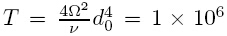 ,where Ω
is the angular speed of rotation around the z-axis,
d0 is the depth of the fluid layer,ν is the fluid kinematic viscosity.The domain is given by
{ x ∈ (0,2),y ∈ (0,2),z ∈ (-1,1)},which is partitioned by 51 × 51 × 51 grids.The grids
are distributed uniformly in each direction.The calculated contours of the sub-grid viscosity
are shown in Figs.1(a)-1(b).
,where Ω
is the angular speed of rotation around the z-axis,
d0 is the depth of the fluid layer,ν is the fluid kinematic viscosity.The domain is given by
{ x ∈ (0,2),y ∈ (0,2),z ∈ (-1,1)},which is partitioned by 51 × 51 × 51 grids.The grids
are distributed uniformly in each direction.The calculated contours of the sub-grid viscosity
are shown in Figs.1(a)-1(b).
| [1] | Zhu, Z. J. Numerical Study of Flows Around Rectangular Cylinders (in Chinese), Ph. D. disser-tation, Shanghai Jiaotong University, 1-22 (1990) |
| [2] | Vickery, B. J. Fluctuating lift and drag on a long cylinder of square cross-section in a smooth and in a turbulent stream. Journal of Fluid Mechanics, 25, 481-494 (1966) |
| [3] | Okajima, A. Strouhal numbers of rectangular cylinders. Journal of Fluid Mechanics, 123, 379-398 (1982) |
| [4] | Bearman, P. W. and Trueman, D. M. An investigation of the flow around rectangular cylinders. Aeronautical Quarterly, 23, 229-237 (1972) |
| [5] | Courchesne, J. and Laneville, A. An experimental evaluation of drag coefficient for rectangular cylinders exposed to grid turbulence. Journal of Fluids Engineering, 104, 523-528 (1982) |
| [6] | Nakamura, Y. and Tomonari, Y. The effect of turbulence on the drags of rectangular prisms. Japan Society of Aeronautical Space Sciences Transactions, 19, 82-86 (1976) |
| [7] | Davis, R. W., Moore, E. F., and Purtell, L. P. A numerical-experimental study on confined flow around rectangular cylinders. Physics of Fluids, 23, 46-59 (1984) |
| [8] | Lyn, D. A. and Rodi, W. The flapping shear layer formed by flow separation from the forward corner of a square cylinder. Journal of Fluid Mechanics, 267, 353-376 (1994) |
| [9] | Gu, Z. F. and Sun, T. F. On interference between two circular cylinders in staggered arrangement at high subcritical Reynolds numbers. Journal of Wind Engineering and Industrial Aerodynamics, 80, 287-309 (1999) |
| [10] | Gu, Z. F. and Sun, T. F. Classifications of flow pattern on three circular cylinders in equilateral-triangular arrangements. Journal of Wind Engineering and Industrial Aerodynamics, 89, 553-568 (2001) |
| [11] | Luo, S. C., Chew, Y. T., and Ng, Y. T. Characteristics of square cylinder wake transition flows. Physics of Fluids, 15, 2549-2559 (2003) |
| [12] | So, R. M. C., Wang, X. Q., Xie, W. C., and Zhu, J. Free-stream turbulence effects on vortex-induced vibration and flow-induced force of an elastic cylinder. Journal of Fluids and Structures, 24, 481-495 (2008) |
| [13] | Zhou, Y. Vortical structures behind three side-by-side. Experiments in Fluids, 34, 68-76 (2003) |
| [14] | Wang, H. F. and Zhou, Y. The finite-length square cylinder near wake. Journal of Fluid Mechanics, 638, 453-490 (2009) |
| [15] | Alam, M. M., Zhou, Y., Zhao, J. M., Flamand, O., and Boujard, O. Classification of the tripped cylinder wake and bi-stable phenomenon. International Journal of Heat and Fluid Flow, 31, 545-560 (2010) |
| [16] | Alam, M. M., Zhou, Y., and Wang, X. W. The wake of two side-by-side square cylinders. Journal of Fluid Mechanics, 669, 432-471 (2011) |
| [17] | Kelkar, K. M. and Patankar, S. V. Numerical prediction of vortex shedding behind a square cylinder. International Journal for Numerical Methods in Fluids, 14, 327-341 (1992) |
| [18] | Robichaux, J., Balachandar, S., and Vanka, S. P. Three-dimensional Floquet instability of the wake of square cylinder. Physics of Fluids, 11, 560-578 (1999) |
| [19] | Williamson, C. H. K. Vortex dynamics in the cylinder wake. Annual Review of Fluid Mechanics, 28, 477-525 (1996) |
| [20] | Bosch, G. and Rodi, W. Simulation of vortex shedding past a square cylinder with different turbulence models. International Journal for Numerical Methods in Fluids, 28, 601-616 (1998) |
| [21] | Kato, M. and Launder, B. E. The modelling of turbulent flow around stationary and vibrating square cylinders. Proceeding of 9th Symposium Turbulent Shear Flows, Kyoto, 10-4-1 (1993) |
| [22] | Sohankar, A., Norberg, C., and Davidson, L. Simulation of three-dimensional flow around a square cylinder at moderate Reynolds numbers. Physics of Fluids, 11, 288-306 (1999) |
| [23] | Tao, W. Q. Numerical Heat Transfer (in Chinese), Xi'an Jiantong University Press, Xi'an (1988) |
| [24] | Patankar, S. V. Numerical Heat Transfer and Fluid Flow, Hemisphere, New York (1980) |
| [25] | Saha, A. K., Biswas, G., andMuralidhar, K. Three-dimensional study of flow past a square cylinder at low Reynolds numbers. International Journal of Heat and Fluid Flow, 24, 54-66 (2003) |
| [26] | Harlow, F. H. and Welch, J. E. Numerical calculation of time dependent viscous incompressible flow of fluid with free surfaces. Physics of Fluids, 8, 2182-2188 (1965) |
| [27] | Niu, J. L. and Zhu, Z. J. Numerical study of three-dimensional flows around two identical square cylinders in staggered arrangements. Physics of Fluids, 18, 044106 (2006) |
| [28] | Niu, J. L., Zhu, Z. J., and Huang, S. H. Numerical study of convective heat transfer from two identical square cylinders submerged in a uniform cross flow. Numerical Heat Transfer, Part A, 50, 21-44 (2006) |
| [29] | Hanjalic, K. One-point closure model for buoyancy-driven turbulent flows. Annual Review of Fluid Mechanics, 34, 321-347 (2002) |
| [30] | Groetzbach, G. Direct numerical simulation of laminar and turbulent Benard convection. Journal of Fluid Mechanics, 119, 27-53 (1982) |
| [31] | Manhart, M. A zonal grid algorithm for DNS of turbulent boundary layers. Computers and Fluids, 33, 435-461 (2004) |
| [32] | Holmes, P., Lumley, J. L., and Berkooz, G. Turbulence, Coherent Structures, Dynamicsal Systems and Symmetry, Cambridge University Press, Cambridge (1996) |
| [33] | Friedrich, R. and Su, M. D. Large eddy simulation of a turbulent wall-bounded shear layer with longitudinal curvature. Lecture Notes in Physics, 170, 196-202 (1982) |
| [34] | McMillan, O. J. and Ferziger, J. H. Direct testing of subgrid-scale models. AIAA Journal, 17, 1340-1346 (1979) |
| [35] | Smagorinsky, J. S. General circulation experiments with the primitive equations, the basic exper-iment. Monthly Weather Review, 91, 99-164 (1963) |
| [36] | Moin, P. and Kim, J. Numerical investigation of turbulent channel flow. Journal of Fluid Mechan-ics, 118, 341-377 (1982) |
| [37] | Madabhushi, R. K. and Vanka, S. P. Large eddy simulation of turbulence-driven secondary flow in a square duct. Physics of Fluidss A: Fluid Dynamics, 3, 2734-2745 (1991) |
| [38] | Su, M. D. and Friedrich, R. Investigation of fully developed turbulent flow in a straight duct with large eddy simulation. Journal of Fluids Engineering, 116, 677-684 (1994) |
| [39] | V azquez, M. S. and Métais, O. Large-eddy simulation of the turbulent flow through a heated square duct. Journal of Fluid Mechanics, 453, 201-238 (2002) |
| [40] | Métais, O. and Lesieur, M. New trend in large eddy simulation of turbulence. Annual Review of Fluid Mechanics, 28, 45-82 (1996) |
| [41] | Pallares, J. and Davidson, L. Large-eddy simulations of turbulent flow in a rotating square duct. Physics of Fluids, 12, 2878-2894 (2000) |
| [42] | Pallares, J. and Davidson, L. Large-eddy simulations of turbulent heat transfer in stationary and rotating square ducts. Physics of Fluids, 14, 2804-2816 (2002) |
| [43] | Germano, M., Piomelli, U., Moin, P., and Cabot, W. H. A dynamic subgrid-scale eddy viscosity model. Physics of Fluidss A: Fluid Dynamics, 3, 1760-1765 (1991) |
| [44] | Lilly, D. K. A proposed modification of the Germano subgrid-scale closure model. Physics of Fluidss A: Fluid Dynamics, 4, 633-635 (1992) |
| [45] | Cui, G. X., Zhou, H. B., Zhang, Z. S., and Shao, L. A new subgrid eddy viscosity model and its application (in Chinese). Chinese Journal of Computer Physics, 21, 289-293 (2004) |
| [46] | Cui, G. X., Xu, C. X., and Zhang, Z. S. Progress in large eddy simulation of turbulent flows (in Chinese). Acta Aerodynamica Sinica, 22, 121-129 (2004) |
| [47] | Vreman, A. W. An eddy-viscosity subgrid-scale model for turbulent shear flow: algebraic theory and applications. Physics of Fluids, 16, 3670-3681 (2004) |
| [48] | Verma, A. and Mahesh, K. A Lagrangian subgrid-scale model with dynamic estimation of La-grangian time scale for large eddy simulation of complex flows. Physics of Fluids, 24, 085101 (2012) |
| [49] | Holm, D. D. Fluctuation effects on 3D Lagrangian mean and Eulerian mean fluid motion. Physica D, 133, 215-269 (1999) |
| [50] | Cheskidov, A., Holm, D. D., Olson, E., and Titi, E. S. On a Leray-伪 model of turbulence. Proceedings of the Royal Society, 461, 629-649 (2005) |
| [51] | Geurts, B. J. and Holm, D. D. Regularization modeling for large-eddy simulation. Physics of Fluids, 15, 13-16 (2003) |
| [52] | van Reeuwijk, M., Jonker, H. J. J., and Hanjalic, K.Wind and boundary layers in Rayleigh-BWnard convection I, analysis and modelling. Physical Review E, 77, 036311 (2008) |
| [53] | van Reeuwijk, M., Jonker, H. J. J., and Hanjalic, K. Leray-伪 simulations of wall-bounded turbulent flows. International Journal of Heat and Fluid Flow, 30, 1044-1053 (2009) |
| [54] | Trias, F. X., Verstappen, R. W. C. P., Gorobets, A., Soria, M., and Oliva, A. Parameter-free symmetry-preserving regularization modeling of a turbulent differentially heated cavity. Comput-ers and Fluids, 39, 1815-1831 (2010) |
| [55] | Verstappen, R. On restraining the production of small scales of motion in a turbulent channel flow. Computers and Fluids, 37, 887-897 (2008) |
| [56] | Chandrasekhar, S. Hydrodynamic and Hydromagnetic Stability, Oxford University Press, Cam-bridge (1961) |
| [57] | Zhou, J., Adrian, R. J., Balachandar, S., and Kendall, T. M. Mechanisms of generating coherent packets of Hairpin vortices in channel flow. Journal of Fluid Mechanics, 387, 353-396 (1999) |
| [58] | Ganapathisubramani, B., Longmire, E. K., and Marusic, I. Experimental investigation of vortex properties in a turbulent boundary layer. Physics of Fluids, 18, 155105 (2006) |
| [59] | Lin, C. and Zhu, Z. Direct numerical simulation of incompressible flows in a zero-pressure gradient turbulent boundary layer. Advances in Applied Mathematics and Mechanics, 2, 503-517 (2010) |
| [60] | Orlanski, I. A simple boundary condition for unbounded flows. Journal of Computational Physics, 21, 251-269 (1976) |
| [61] | Yang, H. X., Chen, T. Y., and Zhu, Z. J. Numerical study of forced turbulent heat convection in a straight square duct. International Journal of Heat and Mass Transfer, 52, 3128-3136 (2009) |
| [62] | Khanafer, K., Vafai, K., and Lightstone, M. Mixed convection heat transfer in two dimensional open-ended enclosures. International Journal of Heat and Mass Transfer, 45, 5171-5190 (2002) |
| [63] | Papanicolaou, E. and Jaluria, Y. Transition to a periodic regime in mixed convection in a square cavity. Journal of Fluid Mechanics, 239, 489-509 (1992) |
| [64] | Nikitin, N. Finite-difference method for incompressible Navier-Stokes equations in arbitrary or-thogonal curvilinear coordinates. Journal of Computational Physics, 217, 759-781 (2006) |
| [65] | Ni, M. J. and Abdou, M. A. A bridge between projection methods and simple type methods for incompressible Navier-Stokes equations. International Journal of Numerical Methods in Engineer-ing, 72, 1490-1512 (2007) |
| [66] | Tian, Z. F., Liang, X., and Yu, P. X. A higher order compact finite difference algorithm for solving the incompressible Navier-Stokes equations. International Jouranl of Numerical Methods in Engineering, 88, 511-532 (2011) |
| [67] | Brown, D. L., Cortez, R., and Minion, M. L. Accurate projection methods for the incompressible Navier-Stokes equations. Journal of Computational Physics, 168, 464-499 (2001) |
| [68] | Zhu, Z. J., Yang, H. X., and Chen, T. Y. Numerical study of turbulent heat and fluid flow in a straight square duct at higher Reynolds numbers. International Jouranal of Heat Mass Transfer, 53, 356-364 (2010) |
| [69] | Baker, T. J., Potential flow calculation by the approximate factorization method. Journal of Computational Physics, 42, 1-19 (1981) |
| [70] | van der Vorst, H. A. BiCGSTAB: a fast and smoothly converging variant of BICG for the solution of non-symmetric linear system. Journal on Scientific and Statistical Computing, 13, 631-644 (1992) |
| [71] | Zhu, Z. J. and Yang, H. X. Numerical investigation of transient laminar natural convection of air in a tall cavity. Heat and Mass Transfer, 39, 579-587 (2003) |
| [72] | Zhu, Z. J. and Yang, H. X. Discrete Hilbert transformation and its application to estimate the wind speed in Hong Kong. Journal of Wind Engineering and Industrial Aerodynamics, 90, 9-18 (2002) |
| [73] | Wu, F. Nonstandard Picture of Turbulence, 2nd ed., 1-30 (2004) http://arXiv:physics/0308012 |
| [74] | Wu, F. Some key concepts in nonstandard analysis theory of turbulence. Chinese Physics Letters, 22, 2604-2607 (2005) |
| [75] | Wu, F. Mathematical concepts and their physical foundation in the nonstandard analysis theory of turbulence. Chinese Physics, 16, 1186-1196 (2007) |
| [76] | Shraiman, B. I. and Siggia, D. E. Scalar turbulence. nature, 405, 639-646 (2000) |
| [77] | Adrian, R. J., Meinhart, C. D., and Tomkins, C. D. Vortex organization in the outer region of the boundary layer. Journal of Fluid Mechanics, 422, 1-54 (2000) |
| [78] | Natrajan, V. K., Wu, Y., and Christensen, K. T. Spatial signatures of retrograde spanwise vortices in wall turbulence. Journal of Fluid Mechanics, 574, 155-167 (2007) |
| [79] | Tennekes, H. and Lumley, J. L. A First Course in Turbulence, MIT Press, Cambridge, 146-195 (1974) |
| [80] | Frisch, U. The Legacy of A. N. Kolmogorov in Turbulence, Cambridge University Press, Cam-brigde, 81-88 (1995) |