 2014, Vol. 35
Shanghai University
Article Information
- D. M. WEI, S. AL-ASHHAB. 2014.
- Similarity solutions for non-Newtonian power-law fluid flow
- Appl. Math. Mech. -Engl. Ed., 35(9): 1155-1166
- http://dx.doi.org/10.1007/s10483-014-1854-6
Article History
- Received 2013-3-18;
- in final form 2014-2-19


2. Department of Mathematics, Al Imam Mohammad Ibn Saud Islamic University, Riyadh 11623, Saudi Arabia
The problem of the boundary-layer flow of non-Newtonian fluids has recently attracted much attention in many fields. Such a problem has many applications in engineering,e.g.,industrial manufacturing processes such as rolling,glass-fiber production,paper production,drawing of plastic films,and metal spinning. The most commonly used model for non-Newtonian fluids is the Ostwald-de Wael model [1, 2, 3, 4, 5].
The existence and uniqueness of this problem have been widely studied [6, 7, 8, 9, 10] . Nachman and Taliaferro [11] established the existence and uniqueness through a Crocco variable formulation. Many numerical approaches were also used to study the problem [12, 13] .Suetal.[14] and Bogn´ar [15] used an Adomian infinite series approach to obtain the analytic and approximate solutions. Howell et al. [16] studied the problem in the context of momentum and heat transfer on a continuously moving surface in the power law fluid.
It is worthwhile mentioning that this so-called power-law problem has been studied in different settings,especially when it comes to the boundary conditions. Many authors used a zero condition at infinity,while others chose to fix some boundary conditions to zero. Some authors regarded several conditions as arbitrary parameters. Many variations of the “eventual ordinary differential equation” representing the power-law problem appeared in the literature. In many cases,the solutions were obtained for a certain range of the parameters representing the boundary conditions or for a certain range of the power-law indexn. This,in fact,shows the richness of the problem and the immense task which would be studied in its full generality.
We note that the power-law problem is characterized by a power-law indexn.When n=1, we have a Newtonian fluid; when n>1,we have a dilatant or shear-thickening fluid; and when 0<n<1,we have a pseudoplastic non-Newtonian shear-thinning fluid.
We study a somewhat simple (relatively speaking) version of the problem (see Eq. (1) below),
considering all possible values of the power-law indexnand all possible values of
ƒ'(0) = .The
existence and uniqueness have not been discussed earlier for the particular boundary conditions
that we use. A transformation in the dependentand independent variables is used to transform
the problem to a finite domain of the independent variable. The solutions are studied for the
case where ƒ''
does not change the sign. Though our approach is basic,it is somewhat novel
since many other authors used different approaches. We emphasize that the underlying ideas
in these approaches may be similar.
.The
existence and uniqueness have not been discussed earlier for the particular boundary conditions
that we use. A transformation in the dependentand independent variables is used to transform
the problem to a finite domain of the independent variable. The solutions are studied for the
case where ƒ''
does not change the sign. Though our approach is basic,it is somewhat novel
since many other authors used different approaches. We emphasize that the underlying ideas
in these approaches may be similar.
The existence and uniqueness are established with the aid of the Picard-Lindel¨of theorem after we take care of the instances where the solutions do not stay bounded and investigate what happens at those instances. It is also established that the solution does not leave the definition domain where we show y'' ≥0 everywhere. By using the transformed equation,we show that when 0<n≤1,a solution that always has a positive curvature exists; while when n>1,the curvature must change the sign.
In Section 2,we make the transformation of the equation that will help in studying the problem and its solutions. In Section 3,we demonstrate the existence of the global solutions with a positive curvature for pseudoplastic fluids,and show that for dilatant fluids,the solutions must change the sign of the curvature in the global domain. In Section 4,we provide numerical solutions for both fluids to demonstrate our results. 2 Transformed equation
We have the following nonlinear boundary value problem:
Here,the derivatives (primes) are taken with respect toη.If ƒ'' >0,then we can drop the absolute value and rewrite (1) as follows: We make the transformationx=1/(η+1),which transforms the domain of the problem from [1,∞)to(0,1] and yields the following equations:
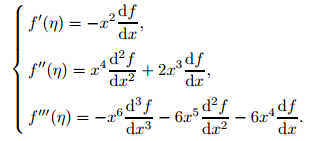
 (note that the two transformations can be combined into one but we keep them separate now). With all derivatives taken with respect tox,wehave
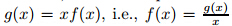
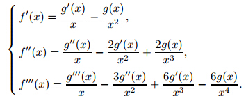


To justify the condition g(0) = 1,notice that ƒ'(η)→1asη→∞transforms to (g(x)−xg'(x)) →1 as x→0. If g'(x) stays bounded asx→0,or more generally,if xg'(x)→0 as x→0,then we can useg(0) = 1 since the limit of g(x) equals 1 as x→0 and wemake the
solution continuous by setting g(0) = 1. Now,we assume that xg'(x)→c≠=0 as x→0. Then,
g'(x) → when g(x) →c+ 1,implying thatg(x) →∞ as x→0. This is a contradiction.
Moreover,the possibility xg'(x) →−∞,g(x) →∞or vice versa will not satisfy the desired
limit since (g(x)− xg'(x))→±∞.
when g(x) →c+ 1,implying thatg(x) →∞ as x→0. This is a contradiction.
Moreover,the possibility xg'(x) →−∞,g(x) →∞or vice versa will not satisfy the desired
limit since (g(x)− xg'(x))→±∞.
In our analysis,we may assume an initial condition g''(1) to replace the condition g(0) = 1, move backwards from 1 to 0,and check whetherx= 0 can be reached withoutggoing to infinity and with g(0) = 1. First,we study the case where g''does not change the sign and is nonnegative. Suppose g'' ≥0. Then,we can drop the absolute value. Therefore,setting y=g(x),we have
subject to

In fact,(4) can be rewritten as a system as follows:

Notice that (4) is singular atx= 0,which is a problem that we shall investigate in our analysis.
Lemma 1 y'' does not change the sign for any solution to(4)for x ∈(0,1) and n<.
Proof Notice that

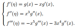
Remark 1 Notice that since ƒ''
(η)=x
3
g''(x),where ƒ''
(η)and g''(x) have the same sign,
for the case ƒ'' <0,if n−1=
 ,then: if bothpandqare odd integers,(4) holds but with a
negative value on the first term; ifpis even and qis odd,(4) holds as it is; ifpis odd and qis
even,(4) holds but with (− y'')1-nreplacing ( y''
)1-n.
,then: if bothpandqare odd integers,(4) holds but with a
negative value on the first term; ifpis even and qis odd,(4) holds as it is; ifpis odd and qis
even,(4) holds but with (− y'')1-nreplacing ( y''
)1-n.
This remark allows the following lemma.
Lemma 2 y'' does not change the sign for any solution to the transformed power law problem (3) for n<1.
The two preceding lemmas justify studying the cases where y''
does not change the sign.
Notice that if = 1,the problem has a trivial solutiony=1−xwith y''=0. If y'' >0 for all
x∈(0,1),then we must have <; while if y'' <0 for all x∈(0,1),then we must have >1.
In this paper,we study the case where y'' is nonnegative.
3 Existence of solutions with non-negative curvature
We begin our study by analyzing two separate cases as follows:
(i) 0≤<.
(ii)<0.
In each of these two cases,we seek to understand the behavior of the solutions to (4) subject
to (5). Before we draw some conclusions regarding those solutions for different values ofn,we
initially study the boundedness of the solutions in the interval (0,1) for 0 <n<1,and then
extend our analysis in the subsequent subsections to all values ofn.
Case (i) 0≤<
In this case,since we have assumed that y''
does not change the sign,we must have y'' ≥0
and 0≤y≤1. We show by the contradiction that y''
does not stay bounded if n< (i.e.,1−3 n>0). Suppose that y'' <Mfor all x∈[0, 1]. Then,
 <0,it is possible in principle for y''
to approach ∞ as the solution crosses
y=0 at x=a≠0 since y''' will change the sign from +∞ to−∞. Of course,in such a case,
the solution for y''
will not be continuous,butyand y' may be continuous. However,we shall
show that in that case,y''
indeed stays bounded when it is crossing the x-axis. Thus,we can
show that for n<1,y''
(x) does not stay bounded asx→0+,and we must have y'' →+∞as
x→0+.
<0,it is possible in principle for y''
to approach ∞ as the solution crosses
y=0 at x=a≠0 since y''' will change the sign from +∞ to−∞. Of course,in such a case,
the solution for y''
will not be continuous,butyand y' may be continuous. However,we shall
show that in that case,y''
indeed stays bounded when it is crossing the x-axis. Thus,we can
show that for n<1,y''
(x) does not stay bounded asx→0+,and we must have y'' →+∞as
x→0+.
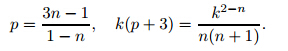
Now,take the case <n<1. In this case,the first termin (4) becomes dominant near
x=0sincey>0. Once again,it is easy to see that it is not possible that y'' →0asx→a+for a≠0. Therefore,y'' stays bounded “away” from x= 0. In fact,asx→0+,one can easily
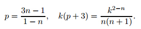
show that y'' →0. More precisely,if we take y''
to be of the order p>0 near x=0,y=1,we
can obtain y'' =kxp
. Substituting the result into the differential equation yields
Case (ii) <0
In this case,since we have assumed that y''
does not change the sign,we must have y'' ≥0
to meet the conditiony(0) = 1,andywill cross thex-axis only once. For the case n<1/3,
just as before and with a similar analysis,we can show that y'' →+∞asx→0+by taking an
“initial condition” for which y>0,saying y(b)=0 where b<a and y(a) = 0. We just need to
rule out the possibility that y'' →∞ when the solution crosses thex-axis at x=a. Insucha
case,y''' will change its sign from +∞ to−∞,and the solution for y''
will not be continuous
(the solution foryand y' may be continuous). However,This will shortly be shown that it does
not happen. Therefore,we need not worry about such solutions. If
<n<1,then just as in
Case (i),y'' →0 as x→0. Therefore,near x=0 and y=1,wehave y'' =kxp,where
Lemma 3 The solutions to(4) subject to(5) satisfy
Now,we show that y''
stays bounded asyapproaches thex-axis for bothn>1andn<1.
First,observe that when −1
 . Equivalently,one can start with
Lemma 4 For the solutions to(4) subject to (5) with <0,the second derivative y'' stays bounded as the solutionycrosses thex-axis and moves back in x.
3.1 Existence and uniqueness for <n<1
Since we have established thaty(x),y'
(x),and y''
(x) stay bounded for all xin (0,1),a
solution to (4) exists for any given initial condition atx= 1. We need to show that there is a
value for y''
(1) for whichy(0) = 1. First,notice that for any 0<b<,a Lipschitz condition
is satisfied on the interval (b,1] so that the existence and uniqueness theorems guarantee the
existence of a unique solution on (b,1]
[17, 18]
. We also obtain that this solution depends continuously on the initial conditions,given for this problem at x= 1. Now,as for the case 0≤<,
notice that the solution where y''
=0 and y' = −s atisfies y(0) =<. Then,we shall show
that a solution exists for whichy(0)>1 so that by the continuity mentioned above,we can
conclude thaty(0) = 1 for some choice of the initial condition y''
(1). Of course,bis chosen to
beclose to 0 so that y'' →0asx→0 will give the required result. Since
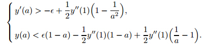 − y''
(1)(1−a). Now,take y''(1) =
− y''
(1)(1−a). Now,take y''(1) = so that y' (a)<−
 . Therefore,y(0)>1,and
For the case <0,we make the following argument. The solution here goes below thex-axis
(i.e.,y<0 on some interval). However,y''
(0) can be chosen large enough so that y(b)=0
for bclose enough tox=1. Since y'''
(x) <0forb<x<,we have y''
(b)>y'' (1). Then,
following our above analysis and by the continuity with respect to the initial condition (i.e.,b is arbitrarily close to 1),we have y(0)>1for y''
(1) large enough.
Theorem 5 There is a unique solution to(4)subject to(5)for < and
<n<1.
3.2 Existence and uniqueness for 0<n<
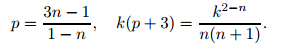
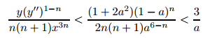
Following a similar analysis as before,we take y'' to be of the order p>0 nearx=0,y=1, i.e.,y'' =kxp. Substituting the above results into the differential equation yields
Integrating from x to 1 yields
 . Notice that to maintain y'' >1,the value ofcx(or kx
3
) will stay to be close to 1 as determined by the value ofn. However,ccan be made arbitrarily close to 1,depending on the value of y''
(1). Therefore,y' (x) can be made arbitrarily small (very negative). In particular,
for a choice of xwhere all the above inequalities hold,we can have
. Notice that to maintain y'' >1,the value ofcx(or kx
3
) will stay to be close to 1 as determined by the value ofn. However,ccan be made arbitrarily close to 1,depending on the value of y''
(1). Therefore,y' (x) can be made arbitrarily small (very negative). In particular,
for a choice of xwhere all the above inequalities hold,we can have
For the case <0,we have y≤0 onsomeinterval(b,1). However,on this interval,y''' <0.
Therefore,y''
(b)>y''
(1). Thus,a similar proof on (0,b) will give the same conclusion. Finally,
observe that forn=
,all the given inequalities hold,and y''
stays bounded in (0,1).
Theorem 6 There is a unique solution to(4)subject to(5)for < and 0<n≤
.
Remark 2 Forn= 0,(4) is undefined. However,(1) has a unique and trivial solution
ƒ'=1 only for = 1. Moreover,though the casen<10 may not have physical significance,
both terms in (4) are negative for−1<n<10,and one can easily show that the solutions fory,
y'
,and y''
cannot stay bounded asx→0+and (5) cannot be met. It can also be easily verified
that the solutions do not stay bounded forn<−1,and the equation is undefined forn=−1.
Therefore,there exists no solution to (4) subject to (5) for < and n<10.
Remark 3 When n= 1,(4) can be rewritten as
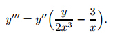
 < and n=1.
3.3 Existence and uniqueness for n=2
< and n=1.
3.3 Existence and uniqueness for n=2When n=2,(4)takesthe form
This equation must have a unique solution in (0,1). However,y'' = 0 is not a solution except when y'' =0 and y= 0,which occurs when y(0) = 0,y'(0) = =0,and y''
(0) = 0.
=0,and y''
(0) = 0.
Now,since y''
does not approach∞in a general solution,the first term in (8) becomes
dominant as we approachx= 0,Eventually,y''
becomes negative. This happens with y>0. If
<0,then this happens afterybecomes positive and the solution crosses thex-axis at some
0<x<,leading toybecoming negative. In a similar fashion,after that y''
andybecome
positive again,if the solutionyhas a limit asx→0,it must be zero. Thus,we have that there
exists no solution to (4) subject to (5) when < and n=2. However,notice that due to the
remark at the end of Section 2,the first term in (8) must change the sign when y'' <0. This
will force the solutions (to the original transformed equation (3)) to terminate. Otherwise,a
contradiction occurs.
Remark 4 The power law equation (2) takes the form ƒ''
ƒ''+
f ƒ''
=0,n=2,which
has a simple solution to meet the boundary conditions when =1 and ƒ''
=0. This solution
is “lost in the simplification process.” In fact,(8) must be multiplied through by y''
(in the
process that leads from (1) to (8)),allowing the solutions to be extended with y''
=0.
Theorem 7 The transformed power-law equation for n=2 which has the form
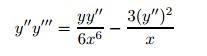 <and y'' ≥0.
Remark 5 The solutions may not be unique if we admit y'' <0. They would have an “alternating behavior” as shown in the MATLAB section. This is also used when n>2(of course the value ofnwill also have to allow y'' <0). 3.4 Existence and uniqueness for 1<n<2
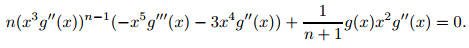
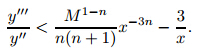
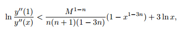
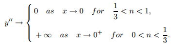
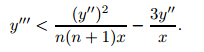
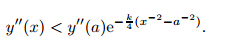
Note that the existence anduniqueness theorems fail at y'' = 0. In this section,our first task is to show by contradiction that y'' does not approach∞asx→0+for positive y(y>δ>0). Suppose that y''' <0 on some interval(0,a)so that
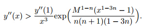
Now,we proceed to show that y'' =0 at some x>0. Since y'' is bounded a bove,the first term in (4) becomes dominant near x= 0. Then,we have
In fact,when y'' reaches 0,it may stay at 0 or proceed according to the given solution and move over to the negative side. Therefore,the solutions need not be unique in this case. However,observe that depending on the value ofn,the above equation may not be satisfied when the right-hand side is negative. Of course,(4) may have to change when y'' <0 as discussed earlier (see the remark at the end of Section 2). But just as before and by continuity with respect to the initial conditions,before y'' reaches 0,we can actually obtain the solutions.
Theorem 8 A unique solution to(4) subject to(5)for which y'' ≥0exists for <1 and
1<n<12.
3.5 Existence and uniqueness for n>2
When n>2,the existence and uniqueness theorems do not hold any longer,and they fail at
y''
= 0. Now,we have y''
in the denominator of the first term in (4). It can easily be shown that
y''
cannot stay bounded and be positive for the solutions to (4). This leads to a contradiction.
Likewise,y''
will not approach ∞ for y>0. Assume that 0≤<,and will move back from 1 to 0. If y''
approaches ∞,y'''
must approach−∞. However,from (4),we have  ,
which implies
,
which implies . The above inequality leads to
 <0,then y''' <0 on(a,0) for some
0<a< where y''
(a)>y''
(1) andy(a) = 0. Then,after a similar analysis,we have that there
exists no solution to (4) subject to (5) for < and n>2.
<0,then y''' <0 on(a,0) for some
0<a< where y''
(a)>y''
(1) andy(a) = 0. Then,after a similar analysis,we have that there
exists no solution to (4) subject to (5) for < and n>2.
Remark 6 As stated before,for the case when n=2,the simplification process leads to
the loss of the solution y''
=0. This is a lsoused for n>2 where the transformed equation (4)
(before simplification) is multiplied through by ( y''
)n−1
. Therefore,we have
Theorem 9 For n>2 and
We have used MATLAB’s ode 45 to numerically confirm our results. Recall that we have
the boundary conditionsy(1) = 0 and y'(1) =− Figure 1 illustrates the existence of the solutions whenn=0.2, Figure 3 shows the alternating curvature behaviors of the solutions whenn=3,
In summary,we have studied the existence and uniqueness of the solutions of the nonlinear
boundary value power-law problem expressed as follows:
<,(9)has a unique solution satisfying(5)and y'' ≥0.
4 Numerical solutions when we use the parameter α for the third
condition y''(1) =α.
=0,and α=0.48.
Figure 2 confirms the existence of the solutions whenn=0.5,=0,and α=0.333 for the case
<n<1.

Fig. 1 Positive curvature withn=0.2,ε=0,
andα=0.48

Fig. 2Positive curvature withn=0.5,ε=0,
andα=0.333 =0,and
α=0.001. Figure 4 shows the alternating curvature behaviors of the solutions whenn=1.4,
=0,and α=0.1. The figures also show that the solutions may not be unique if y'' ≥0 is not
satisfied. Additionally,Fig. 4 shows the sharp turn. It clearly shows that a solution may be
extended when y''
is settled to zero at the “right moment” to reach y=1 at x=0. Ofcourse,
the values of and α have to be correctly chosen.

Fig. 3 Alternating curvature withn=3,ε=0, andα=0.001

Fig. 4 Alternating curvature with n=1.4, ε=0,andα=0.1  ≤1 and for all positive values of the power-law indexnby the classical theorems along
with the Picard-Lindel¨of theorem. The solutions are unique when a nonnegative curvature is
assumed. We have shown theoretically and numerically that for 0<n≤1,the solutions always
have a positive curvature; and for n>1,the curvature must change the sign or be settled to
zero.
≤1 and for all positive values of the power-law indexnby the classical theorems along
with the Picard-Lindel¨of theorem. The solutions are unique when a nonnegative curvature is
assumed. We have shown theoretically and numerically that for 0<n≤1,the solutions always
have a positive curvature; and for n>1,the curvature must change the sign or be settled to
zero.
[1]
Astarita, G. and Marrucci, G. Principles of Non Newtonian Fluid Mechanics, McGraw-Hill Press, New York (1974)
[2]
Schlichting, H. Boundary Layer Theory, McGraw-Hill Press, New York (1979)
[3]
Bohme, G. Non-Newtonian Fluid Mechanics (North-Holland Series in Applied Mathematics and Mechanics), Elsevier, Amsterdam (1987)
[4]
Astin, J., Jones, R. S., and Lockyer, P. Boundary layers in non-Newtonian fluids. Journal de Méchanics, 12, 527-539 (1973)
[5]
Denier, J. P. and Dabrowski, P. On the boundary-layer equations for powerlaw fluids. Proceedings of the Royal Society of London A, 460, 3143-3158 (2004)
[6]
Lu, C. Q. and Zheng, L. C. Similarity solutions of a boundary layer problem in power law fluids through a moving flat plate. International Journal of Pure and Applied Mathematics, 13, 143-166
[7]
Zheng, L., Su, X., and Zhang, X. Similarity solutions for boundary layer flow on a moving surface in an otherwise quiescent fluid medium. International Journal of Pure and Applied Mathematics, 19, 541-552 (2005)
[8]
Guedda, M. Similarity solutions of differential equations for boundary layer approximations in porous media. Journal of Applied Mathematics and Physics, 56, 749-762 (2005)
[9]
Guedda, M. Boundary-layer equations for a power-law shear driven flow over a plane surface of non-Newtonian fluids. Acta Mechanica, 202, 205-211 (2009)
[10]
Guedda, M. and Hammouch, Z. Similarity flow solutions of a non-Newtonian power-law fluid flow. International Journal of Nonlinear Science, 6, 255-264 (2008)
[11]
Nachman, A. and Taliaferro, S. Mass transfer into boundary-layers for power-law fluids. Proceedings of the Royal Society of London A, 365, 313-326 (1979)
[12]
Ece, M. C. and Büyük, E. Similarity solutions for free convection to power-law fluids from a heated vertical plate. Applied Mathematics Letters, 15, 1-5 (2002)
[13]
Liao, S. J. A challenging nonlinear problem for numerical techniques. Journal of Computational Applied Mathematics, 181, 467-472 (2005)
[14]
Su, X., Zheng, L., and Feng, J. Approximate analytical solutions and approximate value of skin friction coefficient for boundary layer of power law fluids. Applied Mathematics and Mechanics (English Edition), 29, 1215-1220 (2008) DOI 10.1007/s10483-008-0910-4
[15]
Bognár, G. Similarity solution of a boundary layer flow for non-Newtonian fluids. International Journal of Nonlinear Sciences and Numerical Simulation, 10, 1555-1566 (2010)
[16]
Howell, T. G., Jeng, D. R., and de Witt, K. J. Momentum and heat transfer on a continuous moving surface in a power-law fluid. International Journal of Heat Mass Transfer, 40, 1853-1861 (1997)
[17]
Arnold, V. I. Ordinary Differential Equations, MIT Press, Cambridge (1978)
[18]
Coddington, E. A. and Levinson, N. Theory of Ordinary Differential Equations, Krieger Publishing Company, Malabar (1984)
