 2014, Vol. 35
Shanghai University
Article Information
- Quan-wen GE. 2014.
- High-order Lagrangian cell-centered conservative scheme on unstructured meshes
- Appl. Math. Mech. -Engl. Ed., 35(9): 1203-1222
- http://dx.doi.org/10.1007/s10483-014-1856-6
Article History
- Received 2013-7-26;
- in final form 2014-1-11


We are chiefly concerned with solving the two-dimensional compressible gas dynamics equation written in the Lagrangian form. In this paper,we intent to construct a high-order Lagrangian cell-centered conservative gas dynamics scheme on unstructured meshes. Before we formulate our algorithm,we briefly review the Lagrangian gas dynamics algorithm.
A Lagrange fluid mechanics algorithm is featured by the cell with the fluid motion,which means that the cell vertices advance with a computed velocity,and the cell face is determined by the vertex location. This guarantees that there is no mass flux passing through the boundary of the Lagrangian moving cell. The Lagrangian fluid dynamics algorithm can ferret out contact discontinuities in the multi-material flow. However,in the Lagrangian framework,the numerical fluxes of the physical conservation laws must be compatible with the vertex velocity computation. The algorithm to meet this requirement is to use a staggered discretization in which the position,velocity,and kinetic energy are centered at the points,while the density, pressure,and internal energy are within the cells. The dissipation of kinetic energy into internal energy through shock waves is guaranteed by an artificial viscosity term. Based on the pioneering work of von Neumann and Richtmyer[1] and Wilkins[2],many Lagrangian staggered discretization schemes were developed,which improved the accuracy and the robustness of the Lagrangian staggered discretization scheme[3,4,5],and a compatible staggered discretization deduced total energy conservation scheme in a rigorous manner was constructed[6,7]. Another choice to the previous discretizations is to establish a Lagrangian cell-centered scheme according to the Godunov method[8,9,10,11,12]. Unlike staggered discretizations,cell-centered schemes have the characteristics of conservation,which have no artificial viscosity term,and permit the direct implementation of the conservation remapping method in the context of the arbitrary Lagrangian Eulerian (ALE) algorithm. The major supposition of all of these algorithms is that the cell masses do not vary with time. Caramana et al.[6] extended the idea of a Lagrangian zone mass to define subzonal Lagrangian masses,and eliminated the artificial cell distortion and hourglass type motion generated in the presence of irregular meshes by the correct utilization of subzonal Lagrangian masses and associated densities and pressures. Ge[13] constructed a scheme with the piecewise constant pressure of the cell. In the following,we describe a high-order Lagrangian cell-centered conservative gas dynamics scheme on general polygonal meshes. With the high-order piecewise pressure of the cell constructed by means of the monotonic upwind scheme for conservation laws (MUSCL)[12],the high-order subcell forces are constructed. The vertex velocities are evaluated by means of momentum conservation. A high-order Lagrangian cell-centered conservative gas dynamics scheme on unstructured meshes is performed by means of the Taylor expansion of fluxes in time centered. The remainder of this paper is structured as follows. Previous work is revisited in Section 2. A high-order Lagrangian cell-centered conservative gas dynamics scheme on unstructured meshes is detailed in Section 3. Extensive numerical experiments are reported in Section 4. Conclusions are given in Section 5. 2 Notation and previous work 2.1 Lagrangian hydrodynamics
We discretize the following equations of the Lagrangian hydrodynamics:
where d/ dt expresses the time derivative. V (t) expresses the control volume,and S(t) expresses its boundary. ρ,U = (u,v)T,P,and E are the density,velocity,pressure,and specific total energy of the fluid,respectively. N expresses the unit outward normal vector to the moving boundary S(t). Equations (1),(3),and (4) indicate the conservation of mass,momentum,and total energy. Equation (2) is also named as the geometric conservation law (GCL). It can also be expressed as the local kinematic equation where X expresses the coordinates defining the control volume surface at time t > 0,and x expresses the coordinates at time t = 0. Then,X = X(x,t) can be implicitly determined by the local kinematic equation,which is also named as the trajectory equation. The equation of state is where ε = E − 1/ 2||U||2. 2.2 Notation and assumptions


Let us consider the physical domain V (0) that is initially filled with the fluid. It is mapped by a set of polygonal cells Ωc (c = 1,2,· · · ,I) without voids or superpositions,where I is the total number of the cells. Each cell is designated by an index c,and is expressed by Ωc. Each vertex of the cell Ωc is designated by an index p. We express by p(c) the counter clockwise ordered list of the points of the cell. The vertices of the cell Ωc satisfy periodicity,i.e.,pp(c)+1 = p1. We express by c(p) the counter clockwise ordered list of the set of the cell around the vertex p. c(p) satisfies periodicity,i.e.,Ωc(p)+1 = Ω1. p− and p+ express the previous and next points with respect to p in the ordered list of the cell vertices (see Fig. 1).
 |
| Fig. 1 Localization of nodal pressures given by half Riemann problems at point p viewed from cell Ωc |
Maire[14] discretized the momentum flux by introducing two pressures  and
and  at each
node p of the cell Ωc (see Fig. 1). Using these nodal pressures,Maire[14] constructed a high-order
cell-centered Lagrangian scheme for two-dimensional compressible fluid flows on unstructured
meshes.
at each
node p of the cell Ωc (see Fig. 1). Using these nodal pressures,Maire[14] constructed a high-order
cell-centered Lagrangian scheme for two-dimensional compressible fluid flows on unstructured
meshes.


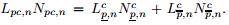 Mpc,n is a 2 × 2 matrix expressed by

Set

Then,
Maire[14] claimed that if (9) was satisfied,then the momentum and total energy could be conserved. However,we find that (9) is incorrect,because Maire[14] introduced two pressures at each node p of the cell Ωc while the pressure discontinuous line exists pqc inside the cell Ωc (see Fig. 1). Similarly,the pressure discontinuous lines pqc (c = 1,2,· · · ,c(p)) exist inside each cell Ωc (c = 1,2,· · · ,c(p)). Due to the presence of these pressure discontinuous lines pqc (c = 1,2,· · · ,c(p)),(9) is incorrect. 3 Conservative spatial approximation 3.1 Compatible discretization of GCL
According to Fig. 2,(2) over the cell Ωc can be rewritten as
where ∂Ωc is the boundary of Ωc,N is the unit outward normal to ∂Ωc,and s is the length element on ∂Ωc. Introduce the discrete divergence operator over cell Ωc as follows: The volume of the cell Ωc,Vc,is a function of the coordinate Xp of the point p for p ∈ p(c). We compute this volume by performing the triangular decomposition of the cell Ωc displayed in Fig. 2.

 |
| Fig. 2 Triangular decomposition of pentagonal cell Ωc |


 |
| Fig. 3 Localization of piecewise pressure viewed from cell Ωc |
We next define what is meant by a piecewise constant pressure of a polygonal cell Ωc.
Although these expositions are given according to a quadrilateral cell in two dimension,all of the
expositions are used to any type of cells in any dimension. In Fig. 3,we show a quadrilateral cell
Ωc,and pick out one of its defining vertices p. We label the side midpoints of a given cell Ωc as
b1,b2,b3,and b4,respectively. Employing the cell vertices p,p+,pk,and p−,the side midpoints
b1,b2,b3,and b4,and the center point c of the cell Ωc,we can partition a quadrilateral Ωc into
four quadrilateral subcells cb1pb2,cb2p+b3,cb3pkb4,and cb4p−b1. Considering the quadrilateral
subcells cb1pb2,cb2p+b3,cb3pkb4,and cb4p−b1,we can express the pressure by
 (p =
1,2,· · · ,p(c)). Then,the pressure of the cell Ωc can be expressed as piecewise constant pressures
(p = 1,2,· · · ,p(c)) in the quadrilateral subcells cb1pb2,cb2p+b3,cb3pkb4,and cb4p−b1. We
know the density ρc,0 and the coordinates of the vertices (Xp,0,Yp,0) (p = 1,2,· · · ,p(c)) of
each cell Ωc at the initial time. We calculate the quadrilateral subcell volumes
(p =
1,2,· · · ,p(c)). Then,the pressure of the cell Ωc can be expressed as piecewise constant pressures
(p = 1,2,· · · ,p(c)) in the quadrilateral subcells cb1pb2,cb2p+b3,cb3pkb4,and cb4p−b1. We
know the density ρc,0 and the coordinates of the vertices (Xp,0,Yp,0) (p = 1,2,· · · ,p(c)) of
each cell Ωc at the initial time. We calculate the quadrilateral subcell volumes
 (p =
1,2,· · · ,p(c)) at the initial time. We calculate the quadrilateral subcell masses
(p =
1,2,· · · ,p(c)) at the initial time. We calculate the quadrilateral subcell masses
 (p = 1,2,· · · ,p(c)) from the initial density ρc,0 and the initial quadrilateral subcell volumes
(p = 1,2,· · · ,p(c)). Then,we know the fluid variables ρc,n,ac,n,Pc,n and the geometrical
characteristics Xp,n,Yp,n (p = 1,2,· · · ,p(c)). We calculate the current time subcell volumes
(p = 1,2,· · · ,p(c)) from the initial density ρc,0 and the initial quadrilateral subcell volumes
(p = 1,2,· · · ,p(c)). Then,we know the fluid variables ρc,n,ac,n,Pc,n and the geometrical
characteristics Xp,n,Yp,n (p = 1,2,· · · ,p(c)). We calculate the current time subcell volumes (p = 1,2,· · · ,p(c)),the current time subcell densities
 and the current time subcell pressures:


 related to the point p and the cell Ωc by
The length d
related to the point p and the cell Ωc by
The length d
 and the unit outward normal D are related to the edge cb1 of the quadrilateral
subcell cb1pb2,and the length d and the unit outward normal D are related to the edge
cb2 of the quadrilateral subcell cb2p+b3. Then,the momentum equation can be written as
To examine momentum conservation,we establish the global balance of momentum without
considering the boundary conditions. The sum of the momentum equation (19) over all the
cells is
Switching the sum over cells and the sum over vertices in the right-hand side,one can obtain
The condition of momentum conservation is
Since the sum of all forces exerting on one point p is equal to zero,the subcell forces satisfy the
condition (22).
3.3 Computation of energy flux
3.4 Construction of solver at vertice velocity Up,n
and the unit outward normal D are related to the edge cb1 of the quadrilateral
subcell cb1pb2,and the length d and the unit outward normal D are related to the edge
cb2 of the quadrilateral subcell cb2p+b3. Then,the momentum equation can be written as
To examine momentum conservation,we establish the global balance of momentum without
considering the boundary conditions. The sum of the momentum equation (19) over all the
cells is
Switching the sum over cells and the sum over vertices in the right-hand side,one can obtain
The condition of momentum conservation is
Since the sum of all forces exerting on one point p is equal to zero,the subcell forces satisfy the
condition (22).
3.3 Computation of energy flux
3.4 Construction of solver at vertice velocity Up,n


We can introduce only one pressure at the point p. This pressure is created by the half Riemann problem defined in the direction of the unit corner vector Npc,n.
where p = 1,2,· · · ,p(c),and Zc is the acoustic impedance of the cell Ωc. The subcell force

 corresponding to the nodal pressure Πpc for each cell Ωc that surrounds
the point p (see Fig. 4) reads
where
corresponding to the nodal pressure Πpc for each cell Ωc that surrounds
the point p (see Fig. 4) reads
where

 is a 2 × 2 symmetric positive definite matrix expressed by

This generic vertex p is not on the boundary of the domain so that it is surrounded by the cells Ωc (c = 1,2,· · · ,c(p)) (see Fig. 4). Since the sum of all forces exerting on one point p is equal to zero,we get

 |
| Fig. 4 Localization of set of cell pressure around vertex p |
 |
| Fig. 5 Localization of sub-cell piecewise pressure around vertex p |


Then,the system satisfied by the point velocity Up,n can be written as
The vector S is defined by


The right-hand sides of (34) are the components of the vector S. The determinant of (34), Δ = AB − C2,is always positive. We have shown that the system (34) can determine the vertex velocity (u*p,n,v*p,n). 3.5 Second-order time discretization
The current paper designs a version of second-order time integration based on the Taylor expansion of the fluxes in time centered. All the physical and geometrical variables are supposed to be known at the beginning of time tn. We express them using the subscript n. Their updated values at time tn+1 = tn + Δt,where Δt is the current time step,are obtained by means of
3.6 Time derivatives of subcell force and nodal velocity
Using the chain rule derivative,we can obtain the time differentiation of (18) as follows:
We calculate the time derivative of the physical variables by utilizing the gas dynamics equations in the non-conservative form: Using the chain rule of derivative,we can obtain the time differentiation of (32) as follows: The corner normal and the corner matrix are expressed as functions of the normal vectors to the two edges of the cell c intersecting at the node p.


where Zc is the acoustic impedance. The time derivative of the corner matrix is calculated by the following chain rule:
As the matrix
 is symmetric and positive definite,(38) gives a unique time derivative for
the nodal velocity.
3.7 Momentum conservation
is symmetric and positive definite,(38) gives a unique time derivative for
the nodal velocity.
3.7 Momentum conservation
Let us write the global balance of momentum without considering the boundary conditions. The sum of the momentum equation (35) over all the cells obtains
Switching the sum over cells and the sum over nodes in the right-hand side of (41),one gains The condition of momentum conservation is Since the sum of all forces intersecting at one point is equal to zero,the condition (43) is satisfied,and the momentum is conserved. 3.8 Boundary conditions


In the Lagrangian formalism,we must consider two types of boundary conditions. One is
that the pressure is imposed on the boundary,and the other is that the normal component of
the velocity is imposed on the boundary. Set p on the boundary. p is arounded by c(p) cells
contained in the domain. There are c(p)+1 edges intersecting at p. They are numbered counter
clockwise (see Fig. 6). The edge [M1,p] of the cell Ω1 is on the boundary. The edge [Mc(p)+1,p]
of the cell Ωc(p) is on the boundary.  and
and  are the outward normals to the two edges
[M1,p] and [Mc(p)+1,p] intersecting at p.
are the outward normals to the two edges
[M1,p] and [Mc(p)+1,p] intersecting at p.
Case 1 A prescribed pressure
Π*1 and Π*c(p)+1 express the pressures that are imposed on the edges [M1,p] and [Mc(p)+1,p] (see Fig. 6). We establish a balance around the vertex p by means of the boundary conditions and conservation relation. Then,we can obtain

 |
| Fig. 6 Notation for boundary conditions |

 is defined by
The right-hand sides of (47) are the components of the vector
is defined by
The right-hand sides of (47) are the components of the vector
 . The system (47) can determine
the velocity (u*p,n,v*p,n).
. The system (47) can determine
the velocity (u*p,n,v*p,n).
The time differentiation of (47) gains

 and
and  are the components of the vector
  defined by

The linear system (48) can provide the time derivative of the vertex velocity ( du*p,n/ dt,dv*p,n/ dt).
Case 2 A prescribed normal velocity
Let W1 and Wc(p)+1 be the values of the prescribed normal velocities on the boundary edges [M1,p] and [Mc(p)+1,p] intersecting at p. We discern the following two cases.
 and
and  are not colinear.
The value of the vertex velocity Up,n is computed by the boundary conditions. The components (u*p,n,v*p,n) of the vertex velocity Up,n are the solution of the following linear system:
The time differentiation of the system (49) obtains This linear system (50) can determine the time derivative of the vertex velocity ( du*p,n/ dt, dv*p,n/ dt). Since the normals are not colinear,the coefficient determinant of the system (50) is not zero.

(ii) and are colinear.
We cannot give directly the vertex velocity Up,n. We need to know the balance around the vertex p which considers the boundary conditions. We gain
After substituting (51) in (52),we can obtain the following equation:


The system satisfied by the vertex velocity Up,n is written as
The vector
 is defined by

where Π* is a mean pressure imposed on the external side of the edges [M1,p] and [Mc(p)+1,p] intersecting at p. We do not know what is the value of the pressure. However,we can build an additional equation by the boundary condition

We obtain
Here,
 and
and
 are the components of the vector
 . We set

The determinant of the liner system (54) is Δ = −AH2 + 2CGH − BG2. Using the fact that AB − C2 > 0,we can obtain Δ < 0. The system (54) can solve the vertex velocity (u*p,n,v*p,n). The time differentiation of (54) obtains
Here,d /
dt and d/
dt are the components of the vector d/
dt defined by
/
dt and d/
dt are the components of the vector d/
dt defined by

The system (55) can determine the time derivative of the vertex velocity ( du*p/ dt,dv*p/ dt). 3.9 Time step
The time step Δt is evaluated by the following criterion. At time tn,for each cell Ωc,we express by λc,n the minimal value of the distance between two vertexes of the cell Ωc. We define
where
 is the maximal value of the local isentropic sound speeds of the quadrilateral subcells
of the cell Ωc.
3.10 Description of algorithm
is the maximal value of the local isentropic sound speeds of the quadrilateral subcells
of the cell Ωc.
3.10 Description of algorithm
(i) Initialization
We know the density ρc,0 and the coordinates of the vertices (Xp,0,Yp,0) (p = 1,2,· · · ,p(c))
of each cell Ωc. We calculate the quadrilateral subcell masses
 (p = 1,2,· · · ,p(c)) from
the initial density ρc,0 and the coordinates of the vertices (Xp,0,Yp,0) of Ωc (p = 1,2,· · · ,p(c),
c = 1,2,· · · ,I). At the time t = tn,we know the fluid variables Uc,n,Ec,n,ρc,n,ac,n,Pc,n and
the geometrical characteristics (Xp,n,Yp,n) (p = 1,2,· · · ,p(c)) in each cell Ωc. We calculate the
quadrilateral subcell volumes
(p = 1,2,· · · ,p(c)) from
the initial density ρc,0 and the coordinates of the vertices (Xp,0,Yp,0) of Ωc (p = 1,2,· · · ,p(c),
c = 1,2,· · · ,I). At the time t = tn,we know the fluid variables Uc,n,Ec,n,ρc,n,ac,n,Pc,n and
the geometrical characteristics (Xp,n,Yp,n) (p = 1,2,· · · ,p(c)) in each cell Ωc. We calculate the
quadrilateral subcell volumes
 (p = 1,2,· · · ,p(c)) and the densities of quadrilateral subcells
 (p = 1,2,· · · ,p(c)). Using the pressure Pc,n and the densities of the quadrilateral subcells
(p = 1,2,· · · ,p(c)),we can get the isentropic sound speed of the quadrilateral subcells
(p = 1,2,· · · ,p(c)). Using (15),(17),(18),and (36),we can calculate the high-order subcell
force
(p = 1,2,· · · ,p(c)). Using the pressure Pc,n and the densities of the quadrilateral subcells
(p = 1,2,· · · ,p(c)),we can get the isentropic sound speed of the quadrilateral subcells
(p = 1,2,· · · ,p(c)). Using (15),(17),(18),and (36),we can calculate the high-order subcell
force
 and the time differentiation of the high-order subcell force d/
dt .
and the time differentiation of the high-order subcell force d/
dt .
(ii) Nodal solver
For each internal vertex,we calculate the velocity (u*p,n,v*p,n) and the time differentiation of the velocity ( du*p,n/ dt,dv*p,n/ dt) by solving the linear system (34) and (38). For each boundary vertex,we calculate the velocity (u*p,n,v*p,n) and the time differentiation of the velocity ( du*p,n/ dt, dv*p,n/ dt) by solving the linear system (47),(48),(49),(50),(54),and (55).
(iii) Time step limitations
We calculate Δt by solving (56).
(iv) Update of the geometrical quantities and the physical variables
We calculate (Xp,n+1,Yp,n+1),τc,n+1,Uc,n+1,and Ec,n+1 from (35).
(v) Equation of state
The internal energy εc,n+1 is given by εc,n+1 = Ec,n+1 − ||Uc,n+1||2/2. Then,we can gain the pressure Pc,n+1 and the isentropic sound speed ac,n+1 from the equation of state. 4 Numerical results 4.1 Shock refraction problem
The computation domain is made up of two adjacent domains. The left border of the first domain is vertical,and the right boundary of the first domain is slanted at an angle of 600 relative to the vertical. The second domain is slanted but uniformly spaced at an angle of 60◦. A reflection boundary condition is imposed on the upper,lower,and right boundaries of the computation domain. The first domain is composed of 30 × 40 cells,and has an initial unit density. The second domain generates unstructured quadrilateral meshes,and has an initial density of 1.5. For the material,we utilize the equation of state of ideal gas (γ = 5/3). The left boundary of the first domain moves at the normal velocity u* p = 1 from left toward right. The problem runs to the time t = 1.3 just before the shock starts to run off the second domain. We show results at this time. In Fig. 7,the initial mesh of a shock refraction problem is shown. In Figs. 8 and 9,the cells at t = 1.3 for the scheme of Maire[14] and a high-order cell-centered conservative scheme are shown. In Figs. 10 and 11,the contour maps of the density at t = 1.3 are shown for the scheme of Maire[14] and a high-order cell-centered conservative scheme. The importance of this problem is that we have both physical vorticity and feigned cell distortion[3,10]. The cell in Fig. 8 is apparently distorted,especially near the lower part of the interface where the cell tends to tangling. The cell in Fig. 9 has not feigned cell distortion and hourglass type motion. The contour map of the density in Fig. 10 does not present physical vorticity. The contour map of the density in Fig. 11 presents physical vorticity. These results do not concede one to discriminate between the two calculations,but the high-order cell-centered conservative scheme is clearly the first rate from the viewpoint of robustness of the computed physical vorticity and the quality of the Lagrangian cell.
 |
| Fig. 7 Initial grid |
 |
| Fig. 8 Cell at time t = 1.3 of scheme of Maire[14] |
 |
| Fig. 9 Cell at time t = 1.3 of high-order Lagrangian cell-centered conservative scheme |
 |
| Fig. 10 Contour map of density at time t = 1.3 of scheme of Maire[14] |
 |
| Fig. 11 Contour map of density at time t = 1.3 of high-order Lagrangian cell-centered conservative scheme |
The computation domain is the quadrilateral (x,y) ∈ [0,1] × [0,0.1]. We use two types of initial cells. The first initial cell is gained by converting regular 50 × 5 cells with the mapping: Xtr = x + (0.1 − y) sin(xπ),Ytr = y. Then,we generate unstructured quadrilateral meshes, unstructured hexagonal meshes,unstructured quadrilateral meshes,and unstructured triangular meshes in the triangle A1A2A3,the quadrilateral A2A4A5A3,the quadrilateral A4A6A7A5, and the triangle A7A6A8 of the domain. Here,the coordinates of A1,A2,A3,A4,A5,A6,A7, and A8 are (0.24,0.1),(0.3,0),(0.3,0.1),(0.33,0),(0.34,0.1),(0.35,0),(0.35,0.1),and (0.45,0), respectively. The second initial mesh is gained by converting regular 100×10 cells with the map ping: Xtr = x+(0.1−y) sin(xπ),Ytr = y. Then,we generate unstructured quadrilateral meshes, unstructured hexagonal meshes,unstructured quadrilateral meshes,and unstructured triangular meshes in the triangle A1A2A3,the quadrilateral A2A4A5A3,the quadrilateral A4A6A7A5, and the triangle A7A6A8 of the domain. Here,the coordinates of A1,A2,A3,A4,A5,A6,A7, and A8 are (0.24,0.1),(0.3,0),(0.3,0.1),(0.33,0),(0.34,0.1),(0.35,0),(0.35,0.1),and (0.45,0), respectively. For the material,we utilize the equation of state of ideal gas (γ = 5/3). The initial condition is (ρc,0,Pc,0,Uc,0) = (1,0,0). The boundary condition is that there is a normal velocity u* p = 1 (the inflow velocity) at x = 0. All the other boundaries are imposed reflection boundary conditions. In Fig. 12,the first initial mesh is shown. In Fig. 13,the second initial mesh is shown. The analytical solution is a shock wave moving at the speed D = 4/3. The correct answer for the density is 4.0 in the singly shocked region,10.0 in the doubly shocked region,and 20.0 in the triply shocked region. The locations of the shock front are 0.966 667 at t = 0.8 and 0.96 and t = 0.93,respectively. In Figs. 14 and 15,the first cell and a contour map of the density at t = 0.8 are shown for the high-order Larangian cell-centered conservative scheme. In Figs. 16 and 17,the second cell and a contour map of the density at t = 0.8 are shown for the high-order Larangian cell-centered conservative scheme. In Figs. 18 and 19,the first cell and a contour map of the density at t = 0.93 are shown for the high-order Larangian cell-centered conservative scheme. In Figs. 20 and 21,the second cell and a contour map of the density at t = 0.93 are shown for the high-order Larangian cell-centered conservative scheme. The main point of the result comparison is that a high-order cell-centered conservative scheme can remove the artificial cell distortion and hourglass type motion,and the results agree well with the precise solution. Finally,we record in Table 1 the mean value of the location of the shock front at t = 0.8. We use two meshes: the first cell and the second cell. The mean value of the location of the shock front at t = 0.8 with the first cell is 0.967 298 for the high-order Larangian cell-centered conservative scheme. The mean value of the location of the shock front at t = 0.8 with the second cell is 0.966 878 for the high-order Larangian cell-centered conservative scheme. The experimental order of the convergence is 1.58 for the high-order Larangian cell-centered conservative scheme.
 |
| Fig. 12 First initial mesh |
 |
| Fig. 13 Second initial mesh |
 |
| Fig. 14 First mesh at t = 0.8 |
 |
| Fig. 15 Contour map of density at t = 0.8 |
 |
| Fig. 16 Second mesh at t = 0.8 |
 |
| Fig. 17 Contour map of density at t = 0.8 |
 |
| Fig. 18 First mesh at t = 0.93 |
 |
| Fig. 19 Contour map of density at t = 0.93 |
 |
| Fig. 20 Second mesh time t = 0.93 |
 |
| Fig. 21 Contour map of density at t = 0.93 |

We have constructed a high-order Lagrangian cell-centered conservative gas dynamics scheme on polygonal cells. The main features of the algorithm are that the high-order subcell forces are constructed by the piecewise constant pressures of the cell. The high-order Lagrangian cell-centered conservative gas dynamics scheme is constructed by means of the Taylor expansion of the fluxes in time-centered. The numerical results demonstrate that the high-order Lagrangian cell-centered conservative gas dynamics scheme is a genuinely two-dimensional highorder scheme.
| [1] | Von Neumann, J. and Richtmyer, R. D. A method for the numerical calculations of hydrodynamical shocks. Journal of Applied Physics, 21, 232-238 (2009) |
| [2] | Wilkins, M. L. Calculation of elastic plastic flow. Methods in Computationnal Physics, 3, 211-263 (1964) |
| [3] | Caramana, E. J. and Shashkov, M. J. Elimination of artificial grid distorsion and hourglasstype motions by means of Lagrangian subzonal masses and pressures. Journal of Computational Physics, 142, 521-561 (2009) |
| [4] | Caramana, E. J., Shashkov, M. J., and Whalen, P. P. Formulations of artificial viscosity for multidimensional shock wave computations. Journal of Computational Physics, 144, 70-97 (2009) |
| [5] | Campbell, J. C. and Shashov, J. C. A tensor artificial viscosity using a mimetic finite difference algorithm. Journal of Computational Physics, 172, 739-765 (2009) |
| [6] | Caramana, E. J., Burton, D. E., Shashkov, M. J., and Whalen, P. P. The construction of compatible hydrodynamics algorithms utilizing conservation of total energy. Journal of Computational Physics, 146, 227-262 (1998) |
| [7] | Campbell, J. C. and Shashkov, M. J. A compatible Lagrangian hydrodynamics algorithm for unstructured grids. Selcuk Journal of Appllied Mathematics, 4, 53-70 (2003) |
| [8] | Godunov, S. K., Zabrodine, A., Ivanov, M., Kraiko, A., and Prokopov, G. Résolution Numérique des Probl mes Multidimensionnels de la Dynamique des Gaz, Mir, Moscou (1979) |
| [9] | Adessio, F. L., CarrollD, E., Dukowicz, K. K., Johnson, J. N., Kashiwa, B. A., Maltrud, M. E., and Ruppel, H. M. Caveat: a Computer Code for Fluid Dynamics Problems with Large Distortion and Internal Slip, Technical Report LA-10613-MS, Los Alamos National Laboratory, Los Alamos (1986) |
| [10] | Dukowicz, J. K. and Meltz, B. Vorticity errors in multidimensional Lagrangian codes. Journal of Computational Physics, 99, 115-134 (1992) |
| [11] | Despŕes, B. and Mazeran, C. Lagrangian gas dynamics in two dimensions and Lagrangian systems. Archive for Rational Mechanics and Analysis, 178, 327-372 (2005) |
| [12] | Carré, G., Delpino, S., Desprées, B., and Labourasse, E. A cell-centered Lagrangian hydrodynamics scheme in arbitrary dimension. Journal of Computational Physics, 228, 5160-5183 (2009) |
| [13] | Ge, Q. W. A Lagrangian cell-centered conservative scheme. Applied Mathematics and Mechanics (English Edition), 33(10), 1329-1350 (2012) DOI 10.1007/s10483-012-1625-9 |
| [14] | Maire, P. H. A high-order cell-centered Lagrangian scheme for two-dimensional compressible fluid flows on unstructured meshes. Journal of Computational Physics, 228, 2391-2425 (2009) |