 2014, Vol. 35
Shanghai University
Article Information
- Si YUAN, Yan DU, Qin-yan XING, Kang-sheng YE. 2014.
- Self-adaptive one-dimensional nonlinear finite element method based on element energy projection method
- Appl. Math. Mech. -Engl. Ed., 35(10): 1223-1232
- http://dx.doi.org/10.1007/s10483-014-1869-9
Article History
- Received 2013-9-24;
- in final form 2014-3-5


Adaptivity is the modern goal of many successful numerical methods,which is especially true to the finite element method (FEM),one of the most widely used numerical methods in engineering applications. In recent years,the adaptive FEM (AFEM) has gained extensive studies in finding efficient and reliable adaptive techniques,especially for nonlinear FEM. There are substantial differences between the implementations of the conventional FEM and the AFEM. In the conventional FEM,the user provides a mesh and gets an FEM solution on that mesh, while the quality and accuracy of the solution are left to be evaluated by the user. In the AFEM,the user specifies an error tolerance for the solution and gets an FEM solution which satisfies the user-specified error tolerance,while the meshes used are adaptively generated and adjusted by the algorithm automatically to guarantee to produce a satisfactory solution in terms of quality and accuracy.
Inspired by the conventional matrix displacement method in structural analysis [1] and based on the projection theorem in the FEM mathematical theory [2] ,Yuan et al. [3,4] proposed a natural and rational method,which is called the element energy projection (EEP) method,for computation of super-convergent solutions from the results of conventional FEM for various linear ordinary differential equations (ODEs). This method proves to be simple,convenient, and effective,and it can produce super-convergent solutions with high quality for both displacements and derivatives at any point on any element. For one-dimensional C0 problems,the EEP super-convergent displacements of the simplified form (i.e.,with linear test/weight functions) gain convergence at least one order higher than the traditional FEM results [5],while those of the condensed form (i.e.,with the same polynomial degree for both trial and test/weight functions) can even gain the optimum super-convergence order [6] .
The high-quality super-convergent solutions by the EEP method encourage a series of steps [7] towards a new AFEM for various linear ODEs [8] ,in which the EEP super-convergent solutions are used to replace the exact solutions in error estimation,and the error-averaging method is then used to refine the mesh. This new AFEM possesses a number of advantages.
(i) The AFEM is a simple algorithmic strategy. The implementation is simple,straightforward,and hence is easy to be extended to various one-dimensional linear problems,e.g.,system of ODEs,first-order ODEs,etc.
(ii) The AFEM has reliable solution accuracy. The accuracy of the AFEM satisfies the pre-specified error tolerance anywhere on the mesh by the strictest maximum norm,which is rarely shared by other methods.
(iii) The AFEM has efficient mesh refinement. The optimum meshes are adaptively generated by the algorithm to meet the accuracy need of each specific problem with little redundant accuracy on the final meshes.
With a series of attempts and efforts,an effective strategy of adaptivity for various onedimensional linear FEM has been successfully developed and applied to a wide range of ODE problems,e.g.,second-order ODEs by C0 FEM [9,10] ,forth-order ODEs by C1 FEM [11] ,and first-order ODEs by C-1 FEM [12] ,and has also been extended to the two-dimensional FEM for Poisson’s equation,plane problems in elasticity,Mindlin plates and shallow shells [13,14] ,as well as to the three-dimensional FEM for the Poisson’ equation on regular domains [14] .
However,all these successful applications are confined to linear problems,whereas many important engineering problems are nonlinear,which exhibit such a wide variety of different forms and properties that it is extremely difficult,if not impossible at all,to construct super-convergence formulas for each individual nonlinear problem in ODEs. To overcome this difficulty,this paper uses Newton’s method to linearize the nonlinear problems under consideration into series of linear problems,so that the existing EEP method can be directly used and the corresponding AFEM can be implemented. The success of such a technology transfer from linear to nonlinear FEM has formed a unified and versatile nonlinear AFEM. Taking the nonlinear ODE of second-order as the model problem (i.e.,one-dimensional C0 FEM),the present paper first gives an introduction of the EEP formula and the associated AFEM for linear problems,and then describes how the technology transfer from linearity to nonlinearity is made. Fundamental ideas,implementation strategy,and computational algorithm are addressed,and representative numerical examples are given to show the efficiency, stability,versatility,and reliability of the proposed approach. 2 AFEM for one-dimensional linear problems 2.1 Model problem and EEP super-convergent solution
Consider the following second-order linear ODE problem:
where p (> 0),q and ƒ are functions of x,
 and L is the associated self-adjoint linear differential operator.
In this paper,polynomial elements of degree m are used with e representing a typical element. After solving the problem (1) by FEM and obtaining a conventional FEM solution uk for the diplacement,the following formula can be used to calcualte the EEP super-convergent displacement [3] :
where ( )* indicates the super-convergent value,
 1
and 2 are the two end-node coordinates
of the element,( )
a indicates the value taken at an arbitrary interior point x
a ∈ (1,2),N 1
and N2
are the two linear shape functions of the element,and h = 2 − 1. Equation (2) is
the EEP formula of the simplified form for super-convergent displacements. If the solution to
the problem (1) is sufficiently smooth,for elements of degree m,uk
gains,as is well known,
the convergence order of hm+1
on element,whereas the super-convergent solution u*
gains the convergence order of hmin(m+3,2m)
for constant coefficient case and of hmin(m+2,2m) for variable
coefficient case,respectively
[5]
. Therefore,in terms of convergence order,u*
gains at least one
order higher than uk
,which justifies the appoach of the practical error estimation described in
the next subsection.
2.2 Adaptive solution based on EEP method
1
and 2 are the two end-node coordinates
of the element,( )
a indicates the value taken at an arbitrary interior point x
a ∈ (1,2),N 1
and N2
are the two linear shape functions of the element,and h = 2 − 1. Equation (2) is
the EEP formula of the simplified form for super-convergent displacements. If the solution to
the problem (1) is sufficiently smooth,for elements of degree m,uk
gains,as is well known,
the convergence order of hm+1
on element,whereas the super-convergent solution u*
gains the convergence order of hmin(m+3,2m)
for constant coefficient case and of hmin(m+2,2m) for variable
coefficient case,respectively
[5]
. Therefore,in terms of convergence order,u*
gains at least one
order higher than uk
,which justifies the appoach of the practical error estimation described in
the next subsection.
2.2 Adaptive solution based on EEP methodThe goal of the proposed self-adaptive solution is,for a user-specified tolerance T ,to find a sufficiently fine mesh π such that the FEM solution uk obtained on the mesh π satisfies the following maximum norm criteria:
In practice,however,u is generally unavailable,and the EEP solution u* from Eq. (2) gains higher order convergence than uk ,and hence u* is used to replace u,leading to the following stop criteria: If certain element does not satisfy the above criteria,then that element will be subdivided into two elements using the error-averaging method [8] ,in which the inserted point is so positioned that the two areas of error squared on the two sides of the point roughly equal to each other. Therefore,the proposed AFEM based on the EEP method,with Eq. (2) for error estimation and the error-averaging method for element subdivision,can briefly be summarized as the following triple-step procedure: (i) Finite element solution. On the current mesh (the initial one is given by the user),an FEM solution uk of the linear problem is obtained. (ii) Super-convergent solution. The EEP solution u* is calculated using Eq. (2),and the maximum error on each element max |u*−uk| is calculated.

(iii) Mesh refinement. For those elements that Eq. (4) is not satisfied,the error-averaging method is used to subdivide each element into two elements,and consequently a new refined mesh is obtained. Then,the first step is repeated again until all elements satisfy Eq. (4). The above triple-step procedure is straightforward and has been successfully used to various linear ODE problems as long as the corresponding EEP super-convergent formulae are available. Therefore,the EEP method is the key-technology in AFEM. 3 AFEM strategy for nonlinear ODE problems 3.1 Model problem and its weak form
Without loss of generality,consider the following second-order nonlinear ODE problem:
where
 ,and N is the associated nonlinear differential operator. The
nonlinearity lies in the fact that both
,and N is the associated nonlinear differential operator. The
nonlinearity lies in the fact that both  and
and  are functions of u and u'
. For simplicity,linear and homogeneous boundary conditions are adopted.
are functions of u and u'
. For simplicity,linear and homogeneous boundary conditions are adopted.
The corresponding weak form for FEM of the Galerkin type is
where v is the test/weight function. 3.2 Newton iteration based on weak form
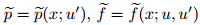
This paper uses Newton’s method to linearize the weak form (6) so that the resulting formulation remains in weak form. Let  denote the FEM solution from
the kth Newton iteration (k = 0 corresponds to the initial solution) and denote the integrand
in Eq. (6) by
denote the FEM solution from
the kth Newton iteration (k = 0 corresponds to the initial solution) and denote the integrand
in Eq. (6) by


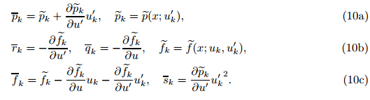
Substituting Eq. (8) into Eq. (6) gives the weak form for the solution uk+1 of the (k + 1)th Newton iteration step
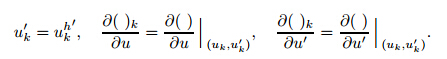
where all the coefficients are linear as follows: Since the solution uk is known from the previous Newton step,all
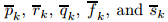 are
functions of x only.
are
functions of x only.
It is easy to see that the weak solution uk+1 from the weak form (9) is equivalent to the solution to the following linear (or linearized) ODE problem:
It is seen that the linearization of the weak form of the nonlinear problem (5) gives the Newton formulation (9) for the weak form,which in turn gives the linear operator form (11). Thus,on the same mesh,the nonlinear FEM solution to the problem (5) has been converted into a series of linear FEM solutions to the problem (11) and is composed of the following steps: substitute the FEM solutions uk and u'k from the kth iteration into Eq. (10) to calculate the coefficients needed in the linearized problem (11); find a new linear FEM solution uk+1 to the linearized problem (11); use the new FEM solution uk+1 to form another linearized problem; and repeat the iteration until two FEM solutions from two adjacent iteration steps are sufficiently close. This iteration of successively upgrading uk+1 on the same mesh is called the nonlinear FEM iteration or Newton iteration. It is noticed that the Newton’s method is both an iteration procedure and a linearization method. 3.3 Technology transfer
After the aforementioned nonlinear FEM iteration,the linearized problem (11) and its FEM solution are obtained,and they are the best linear problem and the best FEM solution on the current mesh since they cannot be improved by further iteration steps unless the mesh is refined. It is at this stage that the linear-problem-based EEP technology can be directly and rightly transferred to the nonlinear problem under consideration to check errors and refine meshes if needed,i.e.,Eq. (2) is used to calculate the EEP solution,which is then used to replace the exact solution in error checking and mesh refinement. For a new mesh thus generated,the nonlinear FEM iteration is restarted followed by the calculation of the EEP solution and mesh refinement if needed,and the procedure is repeated until there is no need for further mesh refinement,i.e., the final mesh and the final FEM solution are obtained. Again,it is noticed that the proposed strategy for nonlinear AFEM does not need to establish formulae of super-convergent solutions for nonlinear problems and,instead,simply makes novel use of the existing AFEM technology for linear problems.
It also needs to note that the linearized problem (11) contains an extra term of  compared
with the problem (1),and it suffices to use
compared
with the problem (1),and it suffices to use  to replace L when calculating the EEP solution in Eq. (2)
[15]
.
3.4 Solution strategy
to replace L when calculating the EEP solution in Eq. (2)
[15]
.
3.4 Solution strategy
From the above,it can be seen that for the nonlinear problem (5),the solution strategy of the EEP-based AFEM also consists of triple steps:
(i) Finite element solution. On the current mesh (the initial one is given by the user),a nonlinear FEM solution uk of the nonlinear problem is obtained,which,on convergence,can also be viewed as a linear FEM solution to the linearized problem (11).
(ii) Super-convergent solution. For the linearized problem (11) and its FEM solution,the EEP solution u* is calculated using Eq. (2),and the maximum error on each element max |u* −uk| is calculated.
(iii) Mesh refinement. The mesh refinement is the same as that for linear problems. It is noticed that for the nonlinear AFEM,the stop criteria are twofold: (i) convergence of nonlinear FEM iteration and (ii) no need for mesh refinement with (i) as a prerequisite. It can also been seen that the difference between the two triple-step procedures for linear and nonlinear cases lies mainly in Step (i),that is,the former is linear,and the latter is nonlinear. 4 Algorithm of one-dimensional nonlinear AFEM
Based on the above discussion,the algorithm of the nonlinear AFEM based on the EEP method can be summarized as follows:
(i) Specify an error tolerance T and an initial mesh π0 on the whole domain (usually a single element is sufficient),and let π* = π0.
(ii) Implement the nonlinear FEM iteration as follows:
(a) Substitute FEM solutions uk and u'k (k = 0,1,2,· · · ,the initial u0 and u'0 are given by user) obtained from the kth nonlinear iteration step into Eq. (10) to form the linearized problem (11).
(b) Solve for the new FEM solution uk+1 and u'k+1 to the problem (11) on the current mesh π*.
Let k := k + 1,if |uk − uk−1| 6 T ,then go to Step (ii),otherwise return to (a) of (ii).
(iii) Implement the error checking and mesh refinement as follows:
(a) For the linearized problem,use Eq.(2) to calculate EEP super-convergent solution u* .
(b) For each element,find e*h,max = max |u* − uk |,and check if Eq. (4) is satisfied. If yes, the corresponding element passes the check. If not,a new interior node is inserted resulting in a new mesh π*.
(iv) If all elements pass,the current mesh is the final mesh,and the solution is finished with current uh being the final FEM solution,otherwise return to Step (ii). 5 Numerical examples
The proposed method can solve various nonlinear problems of the form (5),and in this section,for comparison purpose,some typical numerical examples,especially those with exact solutions available,are given. In all the following examples,a maximum norm is used to control errors,and the specified tolerance is set to be T = 10-6 unless otherwise mentioned. All the initial meshes use a single-element mesh for the whole domain,and the initial solutions are taken simply to be u0 = u'0= 0. Also,m denotes the polynomial degree used by elements,and Ne is the number of elements on the final mesh.
Example 1 Catenary problem
This well-known classic problem can be cast into the following nonlinear ODE problem:
where k is a parameter depending on the length L defined by in the following relation: from which k can be determined once L is given. The exact solution is With L = 2 or L = 3,the exact solutions are shown in Fig. 1. Using the elements of degree m = 2,3,4,the present AFEM results are shown in Table 1.


From the results,it is seen that all the elements of different degrees produce results strictly satisfying the specified error tolerance and the higher polynomial degree the elements use,the fewer elements the final mesh contains. The FEM error variation in the case of L = 2 and m = 4 is shown in Fig. 2,from which it is seen that the proposed method not only can produce results satisfying the specified tolerance,but also can produce roughly uniform error distribution with little accuracy redundancy. This is a desirable feature for a competitive AFEM.
 |
| Fig. 1 Exact solution of Example 1 |
 |
| Fig. 2 Error of Example 1 for L = 2 and m = 4 |

Example 2 Large deflection of semi-infinite membrane This problem,as shown in Fig. 3,can be cast into the following nonlinear ODE problem [16] :
where
 . The exact solution is
and the shape of the deflection is shown in Fig. 4. For this problem,when f < 1,it has a unique
solution; when f > 1,it has no real solution; and f = 1 is the critical load,under which the
derivative of u is infinite at x = 1.
. The exact solution is
and the shape of the deflection is shown in Fig. 4. For this problem,when f < 1,it has a unique
solution; when f > 1,it has no real solution; and f = 1 is the critical load,under which the
derivative of u is infinite at x = 1.

 |
| Fig. 3 Semi-infinite membrane |
 |
| Fig. 4 Exact solution of Example 2 |
Using the elements of degree m = 2,3,4,all the results from the present AFEM satisfy the specified tolerance. Figure 5 gives the AFEM solution with f = 0.9 and m = 2,and the final mesh is plotted on the horizontal axis. The error plot is shown in Fig. 6,and it is seen that the error is well controlled with little accuracy redundancy.
Example 3 Chemical reaction problem
This problem can be cast into the following nonlinear ODE problem [17] :
which has multiple solutions Two solutions for θ are θ1 = 1.517 164 599 and θ2 = 10.938 702 77,respectively,and the two corresponding solutions u1 and u2 are shown in Fig. 7.

 |
| Fig. 5 FEM solution and final mesh for ƒ = 0.9 and m = 2 |
 |
| Fig. 6 Error of Example 2 for ƒ = 0.9 and m = 2 |
 |
| Fig. 7 Two exact solutions of Example 3 |
Taking different initial solutions leads to different final solutions. If u0 = 0,the FEM solution approaches u1. If u0 = 3,the FEM solution approaches u2 . The AFEM errors of both cases satisfy the specified error tolerance with different final meshes as shown in Table 2.

The present paper represents a procedure of the adaptive C0 FEM for nonlinear ODE problems based on the EEP method developed by the research team led by the first author. The method uses Newton’s method to linearize nonlinear problems into a series of linear problems so that the EEP formulation and the corresponding adaptive strategy can be directly used without the need for specific super-convergence formulation for nonlinear FEM. As a result,a unified and general self-adaptive algorithm for nonlinear FEM analysis is established. The procedure has also been extended to other one-dimensional FEM analysis such as the forth-order nonlinear ODE problem and the system of first-order nonlinear ODEs. The full successes in onedimensional nonlinear FEM has paved the way for the further application in two-dimensional nonlinear FEM,for which the original two-dimensional nonlinear problems will be linearized into a series of linear ones,and then these linear two-dimensional problems will be self-adaptively solved using the strategy proposed in Ref. [14]. All of these results will be given in separate papers.
| [1] | Yuan, S. The loss and recovery of stress accuracy in FEM as seen from matrix displacement method (in Chinese). Mechanics in Engineering, 20(4), 1-6 (1998) |
| [2] | Strang, G. and Fix, G. An Analysis of the Finite Element Method, Prentice-Hall, London (1973) |
| [3] | Yuan, S. and Wang, M. An element-energy-projection method for post-computation of super- convergent solutions in one-dimensional FEM (in Chinese). Engineering Mechanics, 21(2), 1-9 (2004) |
| [4] | Yuan, S., Wang, X., Xing, Q. Y., and Ye, K. S. A scheme with optimal order of super-convergence based on the element energy projection method-I formulation (in Chinese). Engineering Mechan- ics, 24(10), 1-5 (2007) |
| [5] | Zhao, Q. H. The Mathematical Analysis on Element Energy Projection Method (in Chinese), Ph. D. dissertation, Hunan University (2007) |
| [6] | Yuan, S. and Zhao, Q. H. A scheme with optimal order of super-convergence based on the element energy projection method-III mathematical analysis (in Chinese). Engineering Mechanics, 24(12), 1-5 (2007) |
| [7] | Yuan, S. and He, X. F. Self-adaptive strategy for one-dimensional finite element method based on element energy projection method. Applied Mathematics and Mechanics (English Edition), 27(11), 1461-1474 (2006) DOI 10.1007/s10483-006-1103-1 |
| [8] | Yuan, S., Xing, Q. Y., Wang, X., and Ye, K. S. Self-adaptive strategy for one-dimensional finite el- ement method based on EEP method with optimal super-convergence order. Applied Mathematics and Mechanics (English Edition), 29(5), 591-602 (2008) DOI 10.1007/s10483-008-0504-8 |
| [9] | Xing, Q. Y. Adaptive Analysis of 1D Galerkin FEM Based on EEP Super-convergent Method (in Chinese), Ph. D. dissertation, Tsinghua University (2008) |
| [10] | Xiao, J. Adaptive FEM Analysis of Second-order ODEs of FEMOL Based on EEP Super- convergent Method (in Chinese), Ph. D. dissertation, Tsinghua University (2009) |
| [11] | Sui, X. Super-Convergent Solutions and Adaptive Analysis of 1D C1 FEM Based on EEP Method (in Chinese), Ph. D. dissertation, Tsinghua University (2010) |
| [12] | Xiao, C. Adaptive FEM Analysis for Systems of First-Order ODEs Based on EEP Super- Convergent Method (in Chinese), Ph. D. dissertation, Tsinghua University (2009) |
| [13] | Fang, N. Adaptive FEMOL Analysis of Elastic Problems Based on EEP Super-Convergent Method (in Chinese), Ph. D. dissertation, Tsinghua University (2011) |
| [14] | Xu, J. J. Research on Adaptive FEM Analysis for 2D and 3D Problems Based on EEP Super- Convergent Method (in Chinese), Ph. D. dissertation, Tsinghua University (2012) |
| [15] | Yuan, S. and Lin, Y. J. An EEP method for post-computation of super-convergent solutions in one-dimensional Galerkin FEM for second order non-self-adjoint boundary-value problem (in Chinese). Chinese Journal of Computational Mechanics, 24(2), 142-147 (2007) |
| [16] | Yuan, S. The Finite Element Method of Lines, Science Press, Beijing/New York, 382-389 (1993) |
| [17] | Ascher, U. Numerical Solution of Boundary Value Problems for Ordinary Differential Equations, Prentice-Hall, New Jersey, 89-90 (1988) |