 2014, Vol. 35
Shanghai University
Article Information
- Yi-rang YUAN, Chang-feng LI, Tong-jun SUN, Yun-xin LIU. 2014.
- Characteristic fractional step finite difference method for nonlinear section coupled system
- Appl. Math. Mech. -Engl. Ed., 35(10): 1311-1330
- http://dx.doi.org/10.1007/s10483-014-1869-9
Article History
- Received 2013-9-30;
- in final form 2014-2-14


2. School of Economics, Shandong University, Jinan 250100, P. R. China
For the nonstationary flow computation of multilayer dynamics of fluids in porous media,we consider a kind of three-layer problems. The flows move horizontally at the first and third layers and move vertically at the middle layer (the weak percolation layer). Here,we need to obtain the solutions to the following three-dimensional convection-dominated diffusion nonlinear section coupled systems with initial-boundary values[1, 2, 3, 4, 5]:
where

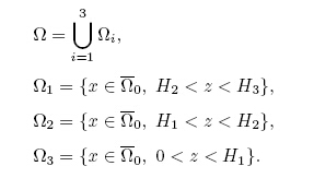
Ω 0 and Ω0 are the base lines of the section and the base region of the three-dimensional problem (see Fig. 1),respectively. ∂Ω and ∂Ω i (i = 1,2,3) are the external boundaries of Ωand Ωi, respectively.
 |
| Fig. 1 Sketch maps |
The initial conditions are

The boundary conditions (the Dirichlet boundary conditions) are

and the interior boundary conditions are

During the simulation of multilayer dynamics of fluids in porous media,these unknown
functions u,w,and v and the potential functions should be computed. Some other functions
Δu,Δv,and ∂w /
∂z denote Darcy’s velocities,Φα (α= 1,2,3) represent the porosity,K1(x,z,u,t),
K2(x,z,w,t),and K3(x,z,v,t) are the stratigraphical permeabilities which are defined in the
model,and a(x,z,u,t) = (a1(x,z,u,t),a2(x,z,u,t))T and b(x,z,v,t) = (b1(x,z,v,t),b2(x,z,
v,t))T,which are the convective coefficients,are given by the following conditions:

Q1(x,z,t,u) and Q3(x,z,t,v) are the external volumetric flow rates.
For convection-diffusion problems,especially those that are convection-dominated,Douglas and Russell[6] have published some famous papers that discuss the characteristic finite difference method and the characteristic finite element method,which are used to overcome oscillation and faults likely arising in the traditional method[1, 7, 8, 9, 10]. Later,Douglas[7] considered the application of the characteristic finite difference method to solve incompressible two-phase dis- placement problems and obtained some convergence results and theoretical foundations by the way of energy mathematics. However,he did not obtain an optimal-order theorem in l2 norm and made it necessary that the problem is -periodic. The authors of this paper have extended Douglas’s results,obtained optimal-order error estimates in l2 norm,and used this method in the numerical simulation of oil deposit and the numerical simulation of enhanced oil recovery simulation[11, 12] with moving boundary value conditions. For large-scale scientific and engi- neering computation (the mode number may amount up to tens of thousands or even hundreds of thousands),fractional step techniques are needed to convert a multi-dimensional problem into a series of successive one-dimensional problems[1, 10, 11, 13]. Though Douglas and Peaceman introduced the alternating-direction method into the two-phase displacement problem,they did not obtain theoretical analysis results. By Fourier analysis,they succeeded in proving the results of stability and convergence of the constant coefficient case,but this method cannot be used for the common equations with variable coefficients[1, 14, 15]. The authors have used the characteristic factional steps method in the compressible two-phase displacement problems and obtained optimal order error estimates in l2 norm. However,the problems should be supposed to be -periodic in the numerical analysis[16].
This paper,in the point of view of the practical exploration and development of oil-gas resources and groundwater percolation computation,discusses the nonstationary flow compu- tation of the multilayer ground percolation coupled system displacement problems. For the nonlinear section coupled system of multilayer fluid dynamics in porous media,a parallel algo- rithm derived by characteristic finite difference fractional steps is stated in this paper. Some techniques,such as calculus of variations,energy methods,twofold-quadratic interpolation of piecewise product type,multiplicative commutation rule of difference operators,decomposition of high order difference operators,and prior estimates are adopted to accomplish the theoretical analysis of optimal order in l2 norm. This problem can be simplified into a two-dimensional expression. Thus,we suppose that the initial problem is linear. We have got some prelimi- nary results[17, 18]. These methods have been used in numerical simulations of multilayer oil resources migration-accumulation problems. Thus,we have thoroughly and completely solved the well-known problem[1, 4, 5, 19, 20, 21, 22].
Generally speaking,this is a positive definite problem as follows:
where Φ∗,Φ∗,K∗,K∗,and A∗ are constants,and the equality K′ 2(w) ≡ 0 holds nearby the planes z = H1 and z = H2.

Our assumption on the regularity of the solutions to (1)-(4) is denoted collectively by

and the functions Q1(x,z,t,u) and Q3(x,z,t,v) are Lipschitz continuous within a distance "0
from the solutions u and v. That is,when |εi| 6 ε0 (1 6 i 6 4),we have

In this paper,M and " express the general positive constant and the general positive small
constant,respectively,and they have different meanings at different places.
2 Second-order characteristic finite difference fractional step scheme
In order to get the solutions by the finite difference method,let the mesh region Ω
0,h replace
Ω0
. On the two-dimensional plane Oxy,let h1 be the step length,xi = ih1,yj = jh1,and let
Ω
0,h replaceΩ
0.

 |
| Fig. 2 Flow model and coordinate system |
Let h2 = (H3 − H2)/N1 (N1 is an integer) be the step length of the partition in the z-axis,zk = H2 + kh2,and tn = nΔt. UseΩ
1,h to replace Ω
1,

Let ∂Ω
1,h and ∂Ω
0,h stand for the boundaries ofΩ
1,h and Ω
0,h,respectively. Similarly,
the length of the partition of Ω
2 in the z-direction is denoted by h3 = (H2 − H1)/N2,and
zk = H1 + kh3. Use Ω
2,h to replace Ω
2,

In Ω
3,the length of the z-direction is taken as h4 = H1/N3,and zk = kh4. Use Ω
3,h to
replace Ω
3,

where N2 and N3 are integers. ∂Ω
2,h and ∂Ω
3,h stand for the external boundaries of Ω
2,h andΩ
3,h,respectively.

Let δx,δz and δx,δz be the forward and backward difference quotients,respectively. dtUn is
the forward quotient of mesh function Un
ik.


As the flow is essentially in the characteristic direction,we use the modified method for the
characteristic procedure to the first-order hyperbolic part of (1a),thus ensuring the high-order
accuracy of numerical results[6, 7, 8, 9]. Let

We write Eq. (1a) in the following form:

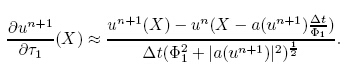
For Eq. (1a),the characteristic finite difference fractional step scheme is given by
where we interpret Un(X) as the piecewise product twofold-quadratic interpolation[8, 9].
For Eq. (1b),the finite difference scheme is

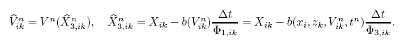
Similarly,let

Then,we rewrite Eq. (1c) as follows:

Approximate δvn+1/
δΤ1
= δv/
δΤ1
(X,tn+1) by a backward difference quotient in the Τ3-direction,

For Eq. (1c),the characteristic finite difference fractional step scheme is given by

The algorithm runs a time interval as follows. Assume that the approximate solution {Un ik,Wn ik,V n ik} at the time level t = tn is known. It is needed to find out the approximate solution {Un+1 ik ,Wn+1 ik ,V n+1 ik } at the next time level t = tn+1. First,by (7a) and (7b),we can get the solution of transition sheaf {U n+1/2 ik } by the method of speedup,take Un+1 i,0 = Wn i,N2 , and obtain the solution {Un+1 ik } by (7c) and (7d). Next,by (9a),(9b),(9c),and (9d),we get the solution of transition sheaf {V n+1/2 ik} and {V n+1 ik} in a similar way. By (8) and the interior boundary conditions (7e) and (9e),we can obtain {Wn+1 ik}. Only in this way can we calculate continuously,so that a complete time step can be carried out. Finally,the positive definite condition guarantees that this difference solution exists,and it is unique. Computation runs for all j in the increasing order from j 1( j ) to j 2( j ) to produce the solutions in the section. Then, the whole approximate solution to the three-dimensional problem can be obtained.
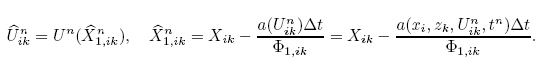
Here,let

where Δt is suitably small. Using the condition of a(X,Un,tn)|δΩ
1 = 0 and b(X,V n,tn)|δΩ
3 =
0,we know that Y = g(X) and Z = f(X) are homeomorphism maps of
Ω1 into
Ω1 and
Ω3
into
Ω3 ,respectively. This can pledge that  and
and  still belong to
Ω1 and
Ω3,and the
Ω-periodic condition can be ignored.
3 Convergence analysis
still belong to
Ω1 and
Ω3,and the
Ω-periodic condition can be ignored.
3 Convergence analysis
Let

Define the inner products on the net function space Hh
[19, 20]. Considering a two-dimensional
mesh region,

The norms on the discrete space are defined by

In general,for brevity,we omit the subscript symbol i of inner products  and norms
Consider (7),(8),and (9) firstly. Let  ,
, ,and
,and  ,where u,v,and
w are exact solutions to the problem (1)-(4),and U,V ,and W are the difference solutions to
(7),(8) and (9),respectively.
,where u,v,and
w are exact solutions to the problem (1)-(4),and U,V ,and W are the difference solutions to
(7),(8) and (9),respectively.
Dispelling Un+1 2 of (7a)-(7e),we get the following equivalent forms:
Next to dispel V n+1 2 of (9a)-(9e),we get the following equivalent forms: Then,we get the error equations of (1)-(4), where where where


Suppose that the space and time steps satisfy

First,consider the error equations (12),and interpret  (X) as the piecewise product
twofold-quadratic interpolation of value {
(X) as the piecewise product
twofold-quadratic interpolation of value { }. Then,


By (12),(15),and (16),we can obtain

Test both sides of (17) against  ,sum it up by parts,and note
the deformation of the second term on the left-hand side,
,sum it up by parts,and note
the deformation of the second term on the left-hand side,

We can obtain


Estimate the third term on the right-hand side of (19),we can obtain
An induction hypothesis is given as follows: For the sixth term on the right hand side of (19),the operators −

 and −
and − are self-conjugate,positive definite,and bounded,and the computational region is a regular
cube,but generally their products vary in a commutative order. Note that
are self-conjugate,positive definite,and bounded,and the computational region is a regular
cube,but generally their products vary in a commutative order. Note that  ,
,
 ,and the flow (the intermediate layer) only moves
vertically. Then,we have
,and the flow (the intermediate layer) only moves
vertically. Then,we have


Owing to the induction hypothesis (23),it is sure that K1(Un)ik,K1(Un)i+1/2 ,k,δxK1(Un)ik, δz(Φ−1 1,ikK1(Un)i+1/ 2 ,k),· · · are bounded. For the first and second terms on the right hand side of (24),owing to the fact that K1(Un) and Φ-1 1 are positive definite and Cauchy inequalities, we can obtain
For the third term,we have Similarly,for the other terms,we can obtain


For the error equation (19),together with (20)-(26),we can obtain
Next,consider the error equation (13). Similarly,we have Testing both sides of (28) against

 and summing it up by parts,
we have
Note that
Together with (30),we can rewrite (29) as follows:
At last,consider the error equations (14). Testing both sides of (14) against δtωn
ik = ωn+1
ik −ωn
ik = dtωn
ikΔt and summing it up by parts,we have
Then,we have
Adding (27),(31),and (33),summing over 0 ≤ n ≤ L,noting the initial conditions
and summing it up by parts,
we have
Note that
Together with (30),we can rewrite (29) as follows:
At last,consider the error equations (14). Testing both sides of (14) against δtωn
ik = ωn+1
ik −ωn
ik = dtωn
ikΔt and summing it up by parts,we have
Then,we have
Adding (27),(31),and (33),summing over 0 ≤ n ≤ L,noting the initial conditions 


 ω0 = 0 and the inequalities

 ,· · · ,we have
where
,· · · ,we have
where
By the discrete Gronwall inequality,we have
At last,it remains to check the induction hypothesis (23). As n = 0,we have = 0.
Thus,the inductive assumption (23) is evidently correct. Assume (23) holds for n = 1,2,· · · ,L.
Let n equal L + 1 and the spacial and temporal parameters satisfy (15). By (35),we have
Then,the induction hypothesis (23) holds as n = L + 1. The proof of (23) is completed.
= 0.
Thus,the inductive assumption (23) is evidently correct. Assume (23) holds for n = 1,2,· · · ,L.
Let n equal L + 1 and the spacial and temporal parameters satisfy (15). By (35),we have
Then,the induction hypothesis (23) holds as n = L + 1. The proof of (23) is completed.

Theorem 1 Suppose that the exact solutions to the problems (1)-(4) satisfy the following
smooth conditions:

Adopt the upwind finite difference fractional steps schemes (7),(8),and (9). Then,the following
error estimate holds:

and the constant M is dependent of the solutions u,v and their derivatives,M∗ =
 .
4 Actual applications
.
4 Actual applicationsRecently,we have introduced these methods into the software system of multilayer oil re- sources migration-accumulation and oil resources estimation of Shengli oil field. The mathe- matical model is
where Ψ o and Ψ w are the potential functions,and kro and krw are the relative permeabilities for oil and water phases,respectively. s′ = ds/dpc,where s is the water concentration,and pc is the capillary pressure. In the simulations,the data of the related parameters can be referred in Table 1

The flow of oil and water migrates and accumulates in the three-dimensional space which proceeds in different directions due to special environments such as geological structures. If the spacial region is divided into lots of sections in suitable direction,the secondary migration- accumulation problems can be similarly interpreted by the sections. Numerical simulation has been done on several sections in the middle Shasan segment of Dongying Hollow.
The industrial district of the middle Shasan region is illustrated by two kinds of vertical sections. One is measured in the east-west direction (named Section I),whose geodetic coor- dinate is from (20 621 246,4 151 110) to (20 641 246,4 151 110). The other is measured from(20 627 246,4 135 110) to (20 627 246,4 153 110) in the south-north direction (named Section II). Their geological structures are displayed in Fig. 3(a) and Fig. 3(b),respectively.
 |
| Fig. 3 Geological structures of Sections I and II |
Then,the numerical simulation results are as follows. The computational parameters are 2 000 meters for the horizontal mesh step,30 for the number of mesh dots in the vertical partitions,and 1 000 years for the temporal step. The computation begins to simulate the migration-accumulation occurring twenty-five million years ago. The initial condition of water flow is assumed to be stationary,and the flow moves outwards on both sides. Numerical results on the 25 million years period include the potentials of water and oil and the concentration of water of different kinds of sections,whose isograms of the present concentration and potential of water and the potential of oil of the East-West sections and the South-North sections are shown in Fig. 4 and Fig. 5,respectively.
 |
| Fig. 4 Isograms of Section I |
 |
| Fig. 5 Isograms of Section II |
The analysis of numerical results is as follows.
(i) The numerical results are reasonable and give expression for the physical-mechanical properties of secondary migration-accumulation. That is to say,oil moves from the higher potential zone to the lower zone,accumulates and shapes a store in the lower potential zones of upper and local tuberositate regions.
(ii) The numerical results depend on the direction choice of sections,and incorrect data might be illustrated due to inappropriate plane cuts of the three-dimensional space.
| [1] | Ewing, R. E. The Mathematics of Reservoir Simulation, SIAM, Philadelphia (1983) |
| [2] | Bredehoeft, J. D. and Pinder, G. F. Digital analysis of areal flow in multiaquifer groundwater systems: a quasi-three-dimensional model. Water Resources Research, 6(3), 883-888 (1970) |
| [3] | Don, W. and Emil, O. F. An iterative quasi-three-dimensional finite element model for heteroge- neous multiaquifer systems. Water Resources Research, 14(5), 943-952 (1978) |
| [4] | Ungerer, P., Dolyiez, B., Chenet, P. Y., Burrus, J., Bessis, F., Lafargue, E., Giroir, G., Heum, O., and Eggen, S. A 2-D model of basin petroleum by two-phase fluid flow, application to some case studies. Migration of Hydrocarbon in Sedimentary Basins (ed. Dolyiez, B.), Editions Techniq, Paris, 414-455 (1987) |
| [5] | Ungerer, P. Fluid flow, hydrocarbon generation and migration. AAPG Bull, 74(3), 309-335 (1990) |
| [6] | Douglas, J. Jr. and Russell, T. F. Numerical method for convection-dominated diffusion prob- lems based on combining the method of characteristics with finite element or finite difference procedures. SIAM J. Numer. Anal., 19(5), 871-885 (1982) |
| [7] | Douglas, J. Jr. Finite difference methods for two-phase incompressible flow in porous media. SIAM J. Numer. Anal., 20(4), 681-696 (1983) |
| [8] | Bermudez, A., Nogueriras, M. R., and Vazquez, C. Numerical analysis of convection-diffusion- reaction problems with higher order characteristics/finite elements, part I: time diseretization. SIAM J. Numer. Anal., 44(5), 1829-1853 (2006) |
| [9] | Bermudez, A., Nogueriras, M. R., and Vazquez, C. Numerical analysis of convection-diffusion- reaction problems with higher order characteristics/finite elements, part II: fuly diseretized scheme and quadratare formulas. SIAM J. Numer. Anal., 44(5), 1854-1876 (2006) |
| [10] | Peaceman, D. W. Fundamental of Numerical Reservoir Simulation, Elsevier, Amsterdam (1980) |
| [11] | Yuan, Y. R. C-F-D method for moving boundary value problem. Science in China, Ser. A, 24(10), 1029-1036 (1994) |
| [12] | Yuan, Y. R. C-F-D method for enhanced oil recovery simulation. Science in China, Ser. A, 36(11), 1296-1307 (1993) |
| [13] | Marchuk, G. I. Splitting and alternating direction method. Handbook of Numerical Analysis (eds. Ciarlet, P. G. and Lions, J. L.), Elesevior Science Publishers, Paris, 197-460 (1990) |
| [14] | Douglas, J. Jr. and Gunn, J. E. Two order correct difference analogous for the equation of multi- dimensional heat flow. Math. Comp., 17(81), 71-80 (1963) |
| [15] | Douglas, J. Jr. and Gunn, J. E. A general formulation of alternating direction methods, part 1. parabolic and hyperbolic problems. Numer. Math., 6(5), 428-453 (1964) |
| [16] | Yuan, Y. R. Fractional steps method. Science in China, Ser. A, 28(10), 893-902 (1998) |
| [17] | Yuan, Y. R. Upwind finite difference fractional steps method. Science in China, Ser. A, 45(5), 578-593 (2002) |
| [18] | Yuan, Y. R. Characteristic fractional step finite difference method. Science in China, Ser. A, 35(11), 1-27 (2005) |
| [19] | Lazarov, R. D., Mischev, I. D., and Vassilevski, P. S. Finite volume methods for convection- diffusion problems. SIAM J. Numer. Anal., 33(1), 31-55 (1996) |
| [20] | Ewing, R. E. Mathematical modeling and simulation for multiphase flow in porous media. Nu- merical Treatment of Multiphase Flows in Porous Media, Springer-Verlag, New York (2000) |
| [21] | Yuan, Y. R. and Han, Y. J. Numerical simulation of migration-accumulation of oil resources. Comput. Geosi., 12, 153-162 (2008) |
| [22] | Yuan, Y. R., Wang, W. Q., and Han, Y. J. Theory, method and application of a numerical simulation in an oil resources basin method of numerical solution of aerodynamic problems. Special Topics & Reviews in Porous Media-An International Journal, 1, 49-66 (2012) |
| [23] | Samarskii, A. A. and Andreev, B. B. Finite Difference Methods for Elliptic Equation, Science Press, Beijing (1994) |
| [24] | Ewing, R. E., Lazarov, R. D., and Vassilev, A. T. Finite difference scheme for parabolic problems on composite grids with refinement in time and space. SIAM J. Numer. Anal., 31(6), 1605-1622 (1994) |