 2014, Vol. 35
Shanghai University
Article Information
- Wei ZHU, Shi SHU, Li-zhi CHENG. 2014.
- First-order optimality condition of basis pursuit denoise problem
- Appl. Math. Mech. -Engl. Ed., 35(10): 1345-1352
- http://dx.doi.org/10.1007/s10483-014-1860-9
Article History
- Received 2013-6-28;
- in final form 2014-2-28


2. Hunan Key Laboratory for Computation and Simulation in Science and Engineering, Xiangtan University, Xiangtan 411105, Hunan Province, P. R. China;
3. Department of Mathematics and Computational Science, College of Science, National University of Defense Technology, Changsha 410073, P. R. China
In this paper,we consider the well-known basis pursuit denoise (BPDN) problem [1] , minimize kxk
where A is a given M × N matrix,b ∈
 M
is an observed vector,x ∈ N
is an unknown
vector,and δ > 0 is a parameter reflecting the noise level. This problem arises from many
applications,such as quantum mechanics
[1]
and compressed sensing
[2,3]
,and has a quite long
research history. We suggest that the interested readers refer to the original papers
[2,3]
for
better understanding. Recently,sparse recovery and compressed sensing,which were led by
Cand`es et al.
[4,5]
,Donoho
[6]
,Yin et al.
[7]
,Cai et al.
[8]
,and Osher et al.
[9]
,are greatly boosting
the research of solving the BPDN problem efficiently when the required size of problem is very large. In the literature,the most famous way to turn the constrained optimization (1) into an
unconstrained version is the penalty method,by which the BPDN problem becomes
min
where µ > 0 is the penalty parameter. Although the unconstrained optimization (2) is a
convex programming which can be solved based on its first-order optimality condition and
by the fixed point iteration method
[10]
,the penalty parameter is unknown and needs to be
carefully chosen for fast convergence. In this paper,by studying the primal-dual relationship
of the problem (1) under the Lagrangian dual analysis framework,we derive a new first-order
optimality condition for the BPDN problem. This condition provides a new approach to choose
the penalty parameters adaptively in the fixed point iteration algorithm. Meanwhile,we extend
this result to matrix completion
[11,12,13,14,15]
which is a new field on the heel of the compressed sensing.
The numerical experiments of sparse vector recovery and low-rank matrix completion show
validity of the theoretic results.
2 Main results
M
is an observed vector,x ∈ N
is an unknown
vector,and δ > 0 is a parameter reflecting the noise level. This problem arises from many
applications,such as quantum mechanics
[1]
and compressed sensing
[2,3]
,and has a quite long
research history. We suggest that the interested readers refer to the original papers
[2,3]
for
better understanding. Recently,sparse recovery and compressed sensing,which were led by
Cand`es et al.
[4,5]
,Donoho
[6]
,Yin et al.
[7]
,Cai et al.
[8]
,and Osher et al.
[9]
,are greatly boosting
the research of solving the BPDN problem efficiently when the required size of problem is very large. In the literature,the most famous way to turn the constrained optimization (1) into an
unconstrained version is the penalty method,by which the BPDN problem becomes
min
where µ > 0 is the penalty parameter. Although the unconstrained optimization (2) is a
convex programming which can be solved based on its first-order optimality condition and
by the fixed point iteration method
[10]
,the penalty parameter is unknown and needs to be
carefully chosen for fast convergence. In this paper,by studying the primal-dual relationship
of the problem (1) under the Lagrangian dual analysis framework,we derive a new first-order
optimality condition for the BPDN problem. This condition provides a new approach to choose
the penalty parameters adaptively in the fixed point iteration algorithm. Meanwhile,we extend
this result to matrix completion
[11,12,13,14,15]
which is a new field on the heel of the compressed sensing.
The numerical experiments of sparse vector recovery and low-rank matrix completion show
validity of the theoretic results.
2 Main results
We begin by introducing some notations used throughout the paper. The l1,l2
,and l∞ norms of a vector x are denoted by  respectively. Define the signum multifunction of a scalar t ∈ as
n
and its sub-differential,we have SGN(x) 
In order not to burden the presentation with too much details,we sometimes shall not explicitly mention the dimensions of variables when without confusion. To build the first-order optimality condition,we need to build two lemmas firstly.
Lemma 1 For every fixed parameter λ > 0,there holds
and Proof We only prove the first statement. The second one can be validated with the similar arguments. Denote f (u,x) = hu,xi − λkxk 1. We need to show that for every fixed vector u satisfying ||u||∞ 6 λ,it holds

 . In fact,by the Cauchy-Schwartz inequality,
we have hu,xi 6 kuk∞kxk
1. Thus,f (u,x) 6 (kuk∞ − λ)kxk
1
,which implies
. In fact,by the Cauchy-Schwartz inequality,
we have hu,xi 6 kuk∞kxk
1. Thus,f (u,x) 6 (kuk∞ − λ)kxk
1
,which implies 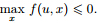 .
Moreover,we have f (u,0) = 0. Therefore,.
.
Moreover,we have f (u,0) = 0. Therefore,.
Lemma 2 The dual problem of BPDN is

Proof By introducing an auxiliary variable r,we can rewrite the BPDN problem in the following equivalent form:

Note that
Therefore,the BPDN problem can be equivalently written as a minimax problem,that is, By the well-known inequality of convex function,we can
deduce the primal-dual relationship [16]
for (7) as follows:
To maximize the objective function in (10),we have to impose a constrained condition on the
variable y from Lemma 1 and avoid the case of taking the value of −∞. More clearly,the
variable needs to satisfy 
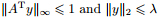 such that
Therefore,the objective function in (10) becomes b
Ty − λσ,which completes the proof.
such that
Therefore,the objective function in (10) becomes b
Ty − λσ,which completes the proof.

Now,we can establish our main results as follows.
Theorem 1 For every fixed parameter σ > 0,any solution x* to the BPDN problem satisfies the following necessary conditions:
with

Proof Let x* be a solution to the BPDN problem and y*
be the dual solution,i.e.,solution to the problem (6). Then,from the preceding arguments,they must satisfy the firstorder optimality conditions of (11) and (12),i.e.,0  There holds


 By the
Slater condition
[17,18]
,there is no duality gap between the primal problem (7) and its problem
(6). Therefore,we have
Thus,it holds
Canceling the variable y*
by (14) and (17),we get
or equivalently
Substituting this expression into (15) and canceling the factor ||Ax* − b||2,we finish the proof of this theorem.
By the
Slater condition
[17,18]
,there is no duality gap between the primal problem (7) and its problem
(6). Therefore,we have
Thus,it holds
Canceling the variable y*
by (14) and (17),we get
or equivalently
Substituting this expression into (15) and canceling the factor ||Ax* − b||2,we finish the proof of this theorem.


Now,let us extend this result to the matrix completion with noise (MCN) [11]
which is on the heel of compressed sensing. Before stating a similar result for the MCN,we need three types of norm of a matrix
 with its singular values {σk
}. The spectral
norm is denoted by kXk and is the largest singular value of X. The Euclidean inner product
between two matrices is hX,Y i := trace(X*
Y ). The corresponding Euclidean norm is called
the Frobenius norm and denoted by
with its singular values {σk
}. The spectral
norm is denoted by kXk and is the largest singular value of X. The Euclidean inner product
between two matrices is hX,Y i := trace(X*
Y ). The corresponding Euclidean norm is called
the Frobenius norm and denoted by  ,that is,=
 . The nuclear norm is
denoted by
. The nuclear norm is
denoted by  and is the sum of singular values. With these notations,we have
the following theorem.
and is the sum of singular values. With these notations,we have
the following theorem.
Theorem 2 For every fixed parameter σ > 0,any solution X* to the MCN problem satisfies the following necessary condition:
with

Proof The proof is similar to that of Theorem 1. 3 Adaptive algorithm 3.1 Fixed point iteration algorithm
The fixed point iteration was proposed in Ref. [10] for the unconstrained minimization (2). The idea behind this iteration is an operator splitting technique. Here,we briefly introduce this iteration for (2). Let us first focus on the first-order necessary condition of (2). Denote y = x − τAT(Ax − b). Then,the condition is equivalent to
for any τ > 0. Note that (22) is a necessary condition for a variable to be an optimality solution to the following convex problem: with v = τ/µ. This problem has a closed form optimal solution given by x = sv (y),where sv (y) is the shrinkage operator given by Thus,the fixed point iteration for (2) is We list the fixed point continuation (FPC) algorithm for (1) as Algorithm 1. Algorithm 1 FPC algorithm


Step (i) Given x0,µ > 0,select µ1 < µ2 < · · · < µL = µ.
Step (ii) Select τ ,and set v = τ/µi and x0 = xi−1.
Step (iii) Compute yk+1 and xk+1 by the iteration formula (25).
Step (iv) Terminate if the stopping criterion is satisfied.
Step (v) Output xi. 3.2 Adaptively fixed point (AFP) iteration algorithm
The continuous technique was adopted in the fixed point iteration algorithm for increasing the penalty parameter µ in Ref. [10] for sparse vector recovery,that is,µi+1 = min{µi ηµ,µ},i =1,2,· · ·,L−1. This updated rule is simple. The penalty parameter at next step is obtained by multiplying a fixed constant ηµ,which is determined by the researchers subjectively,at each outloop. Here,by the first-order optimality condition (13),we design a dynamically updated rule described as follows:
Here,the only difference with the old updated rule lies in that the penalty factor µi ηµ at each outloop has been replaced by µ(xi ) which arises in the new first-order optimality condition. Notice that both the numerator and denominator of µ(xi) decrease as xi tends to the true solution. We modify the dynamically updated rule as
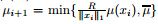 ,where R is
an approximation of the 1-norm of the true solution.
,where R is
an approximation of the 1-norm of the true solution.
We list the AFP iteration algorithm for (1) as Algorithm 2. Algorithm 2 AFP iteration algorithm
Step (i) x0,µ > 0 and the constant R are given as the initial condition.
Step (ii) Compute µi by the updated formula (26).
Step (iii) Select τ ,and set v = τ/µi and x0 = xi−1.
Step (iv) Compute yk+1 and xk+1 by the iteration formula (25).
Step (v) Terminate if the stopping criterion is satisfied.
Step (vi) Output xi.
Finally,we extend this type of algorithm to the MCN. In order to derive a similar iteration, one only needs to know that the following convex problem:
also has a closed form optimal solution [19,20,21] ,which is X = Sv (y),where Sv (y) is the matrix shrinkage operator defined as follows. Given a matrix Y and its reduced singular value decomposition (SVD) given by Y = U diag(
 )VT,Sv (Y ) = U diag()VT with σ = sv (σ). Thus,the
fixed point iteration for the corresponding unconstrained version of (20) is
The remainder computing procedure for the MCN is the same as that for the BPDN problem.
4 Numerical experiments
)VT,Sv (Y ) = U diag()VT with σ = sv (σ). Thus,the
fixed point iteration for the corresponding unconstrained version of (20) is
The remainder computing procedure for the MCN is the same as that for the BPDN problem.
4 Numerical experiments
In this part,two simulation experiments are tested to show the potential of the dynamically
updated rule. One is the sparse vector recovery,and the other is the matrix completion problem.
The codes of the FPC algorithm for the sparse vector recovery and the matrix completion
problem are available. Here,we take comparison between the FPC algorithm and the proposed
AFP algorithm. All the simulations are conducted and timed on a personal computer with an
Intel Pentium-IV CPU 3.06 GHZ and 512 MB memory,running in MA TLAB (version 7.01).
In the first experiment,we test two different scales,1 024 and 2 048,with different ηµ
. The
other parameters are referred to Ref. [22]. From Table 1,one can see that different values of ηµ
have great effects on the CPU time,and our method is comparable to the best result among
them. In the modified dynamically updated rule,we need to estimate the 1-norm of the true
solution x* . If it is known,we take  . Otherwise,we set R = 103
for sparse vector recovery and R = 104 for matrix completion in our simulations.
. Otherwise,we set R = 103
for sparse vector recovery and R = 104 for matrix completion in our simulations.
 |
In the second experiment,we use the default value of ηµ
= 2.0. The scalars,the ranks,the
stop rules,the setting of µ,and the sampling ratios are referred to Ref. [20]. We create random
matrices M ∈ n×m
with rank r by the following procedures. We firstly generate random
matrices ML ∈ n×r
and MR ∈ m×r
with independent and identically distributed Guassian
entries through the MATLAB function randn(·),and then set M = MLM*R
. We sample a
subset Ω through the MATLAB function randsample(·),and the sampled number is cardinality
of Ω,denoted by |Ω|. We test the noiseless case and the noisy case,respectively . In the noisy
case,we corrupt the observations PΩ
(M ) by noise as the following model:


 |
 |
Under the Lagrangian dual analysis framework,we derive a new first-order optimality condition for the BPDN problem. Such a condition provides us with a new approach to choose the penalty parameter adaptively in the fixed point iteration algorithm. Meanwhile,we extend this result to matrix completion. Finally,numerical experiments show validity of the theoretic results.
| [1] | Johnson, B. R., Modisette, J. P., Nordlander, P., and Kinsey, J. L. Wavelet bases in eigenvalue problems in quantum mechanics. APS March Meeting Abstracts, 1, 1903-1903 (1996) |
| [2] | Donoho, D. L. and Elad, M. On the stability of the basis pursuit in the presence of noise. Signal Processing, 86(3), 511-532 (2006) |
| [3] | Chen, S. S., Donoho, D. L., and Saunders, M. A. Atomic decomposition by basis pursuit. SIAM Journal on Scientific Computing, 20(1), 33-61 (1998) |
| [4] | Candès, E. J., Romberg, J. K., and Tao, T. Stable signal recovery from incomplete and inaccurate measurements. Communications on Pure and Applied Mathematics, 59(8), 1207-1223 (2006) |
| [5] | Candès, E. J., Romberg, J., and Tao, T. Robust uncertainty principles: exact signal reconstruction from highly incomplete frequency information. IEEE Transactions on Information Theory, 52(2), 489-509 (2006) |
| [6] | Donoho, D. L. Compressed sensing. IEEE Transactions on Information Theory, 52(4), 1289-1306 (2006) |
| [7] | Yin, W., Osher, S., Goldfarb, D., and Darbon, J. Bregman iterative algorithms for l1-minimization with applications to compressed sensing. SIAM Journal on Imaging Sciences, 1(1), 143-168 (2008) |
| [8] | Cai, J. F., Osher, S., and Shen, Z. Linearized Bregman iterations for compressed sensing. Mathe- matics of Computation, 78(267), 1515-1536 (2009) |
| [9] | Osher, S., Mao, Y., Dong, B., and Yin, W. Fast linearized Bregman iteration for compressive sensing and sparse denoising. Communications in Mathematical Sciences, 8(1), 93-111 (2010) |
| [10] | Hale, E. T., Yin, W., and Zhang, Y. Fixed-point continuation for l1-minimization: methodology and convergence. SIAM Journal on Optimization, 19(3), 1107-1130 (2008) |
| [11] | Candès, E. J. and Plan, Y. Matrix completion with noise. Proceedings of the IEEE, 98(6), 925-936 (2010) |
| [12] | Candès, E. J. and Recht, B. Exact matrix completion via convex optimization. Foundations of Computational Mathematics, 9(6), 717-772 (2009) |
| [13] | Candès, E. J. and Tao, T. The power of convex relaxation: near-optimal matrix completion. IEEE Transactions on Information Theory, 56(5), 2053-2080 (2010) |
| [14] | Zhang, H., Cheng, L., and Zhu, W. Nuclear norm regularization with a low-rank constraint for matrix completion. Inverse Problems, 26(11), 115009 (2010) |
| [15] | Zhang, H., Cheng, L. Z., and Zhu, W. A lower bound guaranteeing exact matrix completion via singular value thresholding algorithm. Applied and Computational Harmonic Analysis, 31(3), 454-459 (2011) |
| [16] | Van Den Berg, E. and Friedlander, M. P. Probing the Pareto frontier for basis pursuit solutions. SIAM Journal on Scientific Computing, 31(2), 890-912 (2008) |
| [17] | Van Den Berg, E. Convex Optimization for Generalized Sparse Recovery, Ph. D. dissertation, the University of British Columbia (2009) |
| [18] | Bertsekas, D. P., Nedic, A., and Ozdaglar, A. E. Convex Analysis and Optimization, Athena Scientific, Belmont (2003) |
| [19] | Cai, J. F., Candès, E. J., and Shen, Z. A singular value thresholding algorithm for matrix com- pletion. SIAM Journal on Optimization, 20(4), 1956-1982 (2010) |
| [20] | Ma, S., Goldfarb, D., and Chen, L. Fixed point and Bregman iterative methods for matrix rank minimization. Mathematical Programming, 128(1-2), 321-353 (2011) |
| [21] | Zhang, H. and Cheng, L. Z. Projected Landweber iteration for matrix completion. Journal of Computational and Applied Mathematics, 235(3), 593-601 (2010) |
| [22] | Hale, E. T., Yin, W. T., and Zhang, Y. A Fixed-Point Continuation Method for l1-Regularized Minimization with Applications to Compressed Sensing, CAAM Technical Report, TR07-07, Rice University, Texas (2007) |