 2015, Vol. 36
Shanghai University
Article Information
- Chao MIN, Nanjing HUANG, Zhibin LIU, Liehui ZHANG. 2015.
- Existence of solutions for implicit fuzzy differential inclusions
- Appl. Math. Mech. -Engl. Ed., 36(3): 401-416
- http://dx.doi.org/10.1007/s10483-015-1914-6
Article History
- Received 2014-04-02;
- in final form 2014-08-15


2. School of Science, Southwest Petroleum University, Chengdu 610500, China;
3. Department of Mathematics, Sichuan University, Chengdu 610064, China
s,distance from the measured position to the bottom along the string;
T,axial tension of the component;
Mt,torque of the string;
N,distributional stress between the string and the hole wall;
Nb,binormal component of N;
Nn,principal normal component of N;
q,linear weight of the string submerged in the drill fluid;
E,Young’s modulus;
I,string inertia moment;
r,string radius;
μ,friction coefficient between the string and the hole wall;
g,unit vector in the gravitational direction;
t,tangential unit vector along the borehole;
n,unit vector in the normal direction of the borehole;
b,unit vector in the binormal direction of the borehole;
kb,curvature of the borehole;
kn,torsion of the borehole;
Mb,flexure moment of the borehole. 1 Introduction
Fuzzy differential equations (FDEs) are useful tool to describe the dynamic performance for the systems with uncertainties. Therefore,it is important to study the solutions of the FDEs in practice[1, 2]. In 1983,Puri and Ralescu[3] introduced the concept of fuzzy valued maps, and employed the Hukuhara derivative (H-derivative) to define the differentiability of fuzzy maps. Thereafter,the theory of FDEs has been extensively developed[4, 5, 6],and the existence and uniqueness of the solutions of FDEs have been widely discussed[7, 8, 9]. However,there still are many open problems. Choudary and Donchev[10] pointed out that the proof of the celebrated theorem of Nieto[11] was not true,making it still an open question that under what conditions, the FDE could have a solution. Kaleva[12] introduced a convergent iteration semigroup of a nonlinear fuzzy-valued function,whose limit function was a solution to an autonomous fuzzy Cauchy problem. Guo et al.[13] discussed the oscillation properties of a class of second-order FDEs with delay,and provided an oscillation criterion. However,it is hard to get the analytic solutions of FDEs. Therefore,numerical methods have also been extensively discussed[14, 15, 16, 17]. The idea of taking the randomness into consideration has received much attention,which might offer a better model for the uncertain dynamical systems[18, 19, 20]. Malinowski[21, 22, 23, 24, 25, 26] discussed the solutions of the random or stochastic FDEs under different conditions.
From the literatures,we can find that there are about five types of methods to research FDEs. The first approach is the classic one,i.e.,the Hukuhara derivative is generalized to a fuzzy valued function. However,in this framework,Diamond[27] pointed out that the diameter of some FDEs’ solution was unbounded with the increase in the time t,which was inconsistent with the crisp cases. The second approach was presented by H¨ullermeier[28]. In his idea,the FDE was replaced by a family of differential inclusions,which overcame the preceding problem. However,the solutions obtained by this method might not be fuzzy valued maps[29, 30]. Combining the idea of Aubin[31, 32],Diamond and Watson[33] exploited this approach by removing the assumption of fuzzy convexity and the compactness of level sets. The third approach is to generalize the differentiability of a fuzzy valued function. Bede et al.[2] and Bede and Gal[34] studied a class of fuzzy initial valued problems (FIVPs) and a class of 2-point boundary value problems with a generalized differentiability,which also allowed to obtain the solutions of FDEs with decreasing diameters. However,there are usually 2 solutions for the FIVPs with respect to this derivative[35, 36, 37, 38]. The fourth approach is to use the parametric representation of fuzzy numbers. Chen et al.[39, 40] proved the existence and uniqueness of the solutions for the fuzzy 2-point boundary value problems based on a redefined differentiability. However,none of the FDEs in this framework possesses a periodic solution. The fifth approach was proposed by Liu[41], where the FDEs were regarded as a type of differential equations,similar to the stochastic differential equation. Thereafter,this method is introduced into the option pricing for fuzzy financial markets[42] and the fuzzy optimal control with application to portfolio selections[43].
In a complex system,it is necessary to treat the qualitative properties. Most of the qualitative problems for FDEs are based on the idea of differential inclusions. Therefore,discussing the solutions of fuzzy differential inclusions (FDIs) is important in the qualitative theory of FDEs. FDIs were first presented by Baidosov[44]. Aubin[32] and Dordan[45] discussed the viability of the FDIs in an equivalent form with toll sets. Lakshmikantham and Mohapatra[30] presented a theorem to show that under what conditions the attainable sets of FDIs are the level sets of a fuzzy map. Zhu and Rao[46] presented two types of FDIs,i.e.,

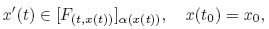
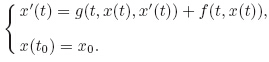
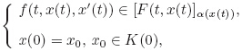
Since the implicit differential equations play an important role in the differential equation theory,it is interesting to generalize the results of Zhu and Rao[46] to the implicit fuzzy differential inclusions (IFDIs) as follows:


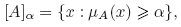
Definition 1 Given a function μA : Rn → [0, 1],a fuzzy set A can be written as {(x,μA) : x ∈ Rn},where μA is called the membership function. For any α ∈ (0,1],we denote the α-level set of A by
A fuzzy set A and its membership function μA are usually taken as one,i.e.,we often simply write the membership of x ∈ Rn in A as A(x). The family of the fuzzy sets on a space X is denoted by F(X).
The space of n-dimensional fuzzy numbers is a set En of the fuzzy sets {u : Rn → [0, 1]}, where u satisfies the following conditions:
(i) There must exist an x ∈ Rn such that u(x0) = 1,i.e.,u is normal.
(ii) u is a fuzzy convex set,which means that for any x,y ∈ Rn and λ ∈ [0, 1],

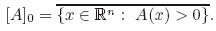
(iii) u is an upper semicontinuous function,which means that [u]α is closed for any α[0, 1].
(iv) [u]0 = {x ∈ Rn : u(x) > 0}is a compact set.
It is obvious that,for each u ∈ En and any α ∈ [0, 1],[u]α is a convex compact subset of
Rn.
The extension principle[47] is presented to extend a crisp function f: X → Y to its fuzzy
situation,i.e.,a fuzzy function
Therefore,we can define the addition operator between a crisp vector a ∈ Rn and a fuzzy
set u ∈ En as a ⊕ u,that is,for any x ∈ Rn,
It is obvious that [a⊕u]α = a+ [u]α,where the addition on the right-hand side of the
equation is the Minkowski sum. Throughout this paper,we denote the sum between a vector
and a fuzzy set,a ⊕ u,by a + u without confusion.
Let BX be the unit ball of a metric space X. BX(x,η) denotes the ball in X centered at x
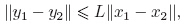
with the radius η. A function f : X → R is said to be Lipschitzean with a constant L > 0 if
for any x,y ∈ X,
Definition 2 If F : X → Y,where X and Y are both metric spaces,F is said to be
Lipschitzean if and only if there exists a constant L ≥ 0 such that
Moreover,a fuzzy function F : X → En is said to be Lipschitzean if there exists a constant
L such that for any α ∈ [0, 1],the set-valued map [F]α is L-Lipschitzean.
Remark 1 We notice that a fuzzy map F : X → En can generate a real valued function
A set-valued map F : X → Y is strict if its domain
Definition 3 (i) For a metric space X,we say that a set-valued map F : X → Y is upper
semicontinuous at x ∈ X if and only if for any neighbourhood U of F(x),there exists an η > 0
such that for all x'∈ BX(x,η),F(x') ⊂
U. Moreover,if F is upper semicontinuous at any
point of X,we say that F is upper semicontinuous.
(ii) We say that a set-valued map F is lower semicontinuous at x ∈ Dom(F) if and only if
for any y ∈ F(x) and any sequence {xn} ⊂ Dom(F) converging to x,there exists a sequence
consisting of the elements yn ∈ F(xn) converging to y. Moreover,if F is lower semicontinuous
at any point x ∈ Dom(F),we say that F is lower semicontinuous.
Contingent cone and contingent derivative are useful tools in the study of the solutions and
the viability of the differential inclusions. Let K be a non-empty set in a Hilbert space,and
the contingent cone TK(x) to K at x be defined as
Lemma 1[48] For a metric space X,let F be a Lipschizean compact convex set-valued map
from X into Rn. If for some M,each x ∈ X,and F(x) ⊂
MB,then F has a Lipschizean
selection f : X → Rn with a Lipschiz constant K.
Now,we present the following existence theorem by Lemma 1 under some strong conditions.
The cases under weakened conditions will be discussed later.
Theorem 1 For an open subset Ω ⊂ R×Rn and (t0,x0) ∈ Ω,assume that the fuzzy map
F : Ω → En is Lipschitzean,and the Lipschitz constant is denoted by L > 0. If there exists some
constant M such that [F(x)]0 ⊂ MB,and the function g : Ω × Rn → Rn satisfies the Lipschitz
condition that there is a neighborhood V = {(t,x,y) ∈ Ω×Rn,|| t−t0||≤a,
||x−x0≤b},then,
Proof First of all,we define the set-valued map
As F(t,x) ∈ En and the elements in En are upper semicontinuous,[F(t,x)]α(x) is a closed
subset of the compact set [F(t,x)]0. Therefore,[F(t,x)]α(x) is also compact. Overall,we can
see that
By Lemma 1,
Denote the ball in Rn by
Next,we will prove that T is a contractive map. Actually,∀φψ ∈ U and ∀t ∈ [t0,t0 + a],
Remark 2 From the proof of the above theorem,we can see that the Lipschitz constant
L2 of g with respect to y is necessarily less than 1. From the routine of the proof,we only need
the selection f of
Next,we will consider the IFDI in an open case,i.e.,
Definition 4 [46] If there exists a constant L > 0 for a fuzzy map F : Ω → En such that
for any (t,x1),(t,x2) ∈ Ω,x1 ≠ x2,y1,y2 ∈ Rn,F(t,x1,y1 : F(X) → F(Y) is defined as follows:


 : X × Rn → [0, 1],where for any x ∈ X and y ∈ Rn,(x,y) = F(x)(y). For convenience,we
do not distinguish F and in the following discussion,and denote them both by F.
: X × Rn → [0, 1],where for any x ∈ X and y ∈ Rn,(x,y) = F(x)(y). For convenience,we
do not distinguish F and in the following discussion,and denote them both by F.


 : Ω → Rn by
 (t,x) is nonempty. By the convexity
of F,we have that,for any u,v ∈(t,x) and λ ∈ [0, 1],
(t,x) is nonempty. By the convexity
of F,we have that,for any u,v ∈(t,x) and λ ∈ [0, 1],
 (·,·) is nonempty and convex.
is a nonempty compact convex valued map from Ω into Rn. Moreover,it is also
Lipschitzean with the Lipschitz constant L.
has a Lipschitzean selection f : Ω → Rn such that f(t,x) ∈ (t,x). We
should notice that the Lipschitz constant denoted by K of f might be different with L. Thus,
it suffices to verify the existence of the solution of the following implicit initial value problem
(IIVP):
(·,·) is nonempty and convex.
is a nonempty compact convex valued map from Ω into Rn. Moreover,it is also
Lipschitzean with the Lipschitz constant L.
has a Lipschitzean selection f : Ω → Rn such that f(t,x) ∈ (t,x). We
should notice that the Lipschitz constant denoted by K of f might be different with L. Thus,
it suffices to verify the existence of the solution of the following implicit initial value problem
(IIVP):


 to be Lipschitzean on some neighborhood. Thus,the condition of F can
be weakened.
to be Lipschitzean on some neighborhood. Thus,the condition of F can
be weakened.


Lemma 2 [49] For a paracompact Hausdorff topological space D and a topological vector space Y,F : D → 2Y is a nonempty convex valued map. If for any y ∈ Y,F−1(y) = {x ∈ D| y ∈ F(x)} is open in D,i.e.,F has open lower sections,then F has a continuous selection f : D → Y such that ∀x ∈ D,f(x) ∈ F(x).
Theorem 2 For an open subset Ω ⊂ R × Rn,(t0,x0) ∈ Ω,and an F-Lipschitzean fuzzy map F : Ω → En with the constant K,suppose that the corresponding function F(t,x,y) : Ω × Rn → [0, 1] is lower semicontinuous at (t,x) ∈ Ω. Suppose that the continuous function g : Ω × Rn → Rn satisfies the same Lipschitz condition (L) in Theorem 1. Let α : Rn → [0,1) be an upper semicontinuous function. Then,we have that on some interval I = [t0,t0 + T], there exists a continuous differentiable function x : I → Rn,which is the solution of (2).
Proof Similar to the proof of Theorem 1,we first define the set-valued map : Ω → Rn
as
 (t,x) is nonempty and
convex.
(t,x) is nonempty and
convex.
For any y ∈ Rn,we assert that −1(y) = {(t,x) ∈ Ω,F(t,x,y) > α(x)} is open in Rn. It
is sufficient to verify that ( −1(y))c = {(t,x) ∈ Ω,F(t,x,y) ≤α(x)} is closed. In fact,for any
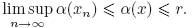
{(tn,xn)} ⊂ ( −1(y))c,we have F(tn,xn,y) ≤ α(xn). Let (tn,xn,y) → (t,x) as n→∞. By the
lower semicontinuity of F(·,·,y) and the upper semicontinuity of α(·),we have
 −1(y))c is closed,and is a nonempty convex set-valued map with open lower sections.
By Lemma 2,there exists a continuous selection f : Ω → Rn of such that,for each (t,x) ∈ Ω,
f(t,x) ∈ (t,x). By the F-Lipschitzean condition of F,f is obviously Lipschitzean with the
Lipschitz constant K. Thus,the solution of the following IIVP is also the solution of (2):
−1(y))c is closed,and is a nonempty convex set-valued map with open lower sections.
By Lemma 2,there exists a continuous selection f : Ω → Rn of such that,for each (t,x) ∈ Ω,
f(t,x) ∈ (t,x). By the F-Lipschitzean condition of F,f is obviously Lipschitzean with the
Lipschitz constant K. Thus,the solution of the following IIVP is also the solution of (2):
The process is similar to the routine in Theorem 1,and thus is omitted here. This completes the proof.
Remark 3 Theorem 2 extends Theorem 4 of Zhu and Rao[46] to an implicit case.
Remark 4 In the first part of the proof above,we should notice that,for any open subset U ⊂ Rn,
 is lower semicontinuous. However,
if is not closed valued,Michael’s selection theorem cannot be applied here.
is lower semicontinuous. However,
if is not closed valued,Michael’s selection theorem cannot be applied here.
Lemma 3 [50] (Michael’s selection theorem) For a metric space X and a Banach space Y, if F : X → Y is a lower semicontinuous closed convex valued map,then F has a continuous selection f : X → Y .
Theorem 3 For an open subset Ω ⊂ R × Rn and (t0,x0) ∈ Ω,suppose that F : Ω → En is an F-Lipschitzean fuzzy map with a constant K,whose corresponding function F(t,x,y) : Ω×Rn → [0, 1] is continuous at (t,x) ∈ Ω and differentiable at y ∈ Rn. The continuous function g : Ω × Rn → Rn satisfies the same Lipschitz condition (L) in Theorem 1. Let α : Rn → (0,1] be an upper semicontinuous function. Assume that the transversality condition is satisfied,i.e., for any (t0,x0) ∈ Ω and y0 ∈ Rn,there exist constants c > 0 and η > 0 such that

Proof Define the set-valued map G(t,x) : Ω → R by
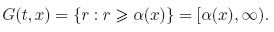
For any z ∈ G(t,x) and TG(t,x)(z) = [α(x) − z,+∞),the transversality condition can be rewritten as follows:
∀(t,x) ∈ B((t0,x0),η),y ∈ B(y0,η),and z ∈ B(F(t0,x0,y0)) ∩ G(t,x),the unit ball of R BR ⊂ cFy'(t,x,BRn) − TG(t,x)(z).
From Theorem 1.5.5 in Ref. [51],we can get that (t,x) is lower semicontinuous,and
 (t,x). Similar to the proof of
Theorem 2,we can get the existence of the solution of (1). This completes the proof.
(t,x). Similar to the proof of
Theorem 2,we can get the existence of the solution of (1). This completes the proof.
In the following theorem,we will discuss the situation when α(x) is lower semicontinuous.
Theorem 4 For an open subset Ω ⊂ R × Rn and (t0,x0) ∈ Ω,suppose that F : Ω → En
is an F-Lipschitzean fuzzy map,whose corresponding function F(t,x,y) : Ω× Rn → [0, 1] is
upper semicontinuous at (t,x) ∈ Ω. The continuous function g : Ω × Rn → Rn satisfies the
same Lipschitz condition (L) in Theorem 1. Let α : Rn → [0,1) be a lower semicontinuous
function. Moreover,if there exists a neighborhood D of (t0,x0) such that  [F(t,x)]α(x) is
compact in Rn,then on some I = [t0,t0 + T],there exists a continuous differentiable function
x : I → Rn,which is the solution of (1).
[F(t,x)]α(x) is
compact in Rn,then on some I = [t0,t0 + T],there exists a continuous differentiable function
x : I → Rn,which is the solution of (1).
Proof Define the set-valued map (t,x) as follows:
 (t,x) is upper semicontiunous on D. By the definition of En,we can clearly
find that (t,x) is nonempty,compact,and convex in Rn. Since R × Rn is locally compact,
for each compact subset K ⊂ D,the graph of the restriction of ,|K : K → Rn,is closed.
Actually,for any Cauchy sequence (tn,xn,yn) ⊂ graph( |K) which converges to (t,x,y),by
(t,x) is upper semicontiunous on D. By the definition of En,we can clearly
find that (t,x) is nonempty,compact,and convex in Rn. Since R × Rn is locally compact,
for each compact subset K ⊂ D,the graph of the restriction of ,|K : K → Rn,is closed.
Actually,for any Cauchy sequence (tn,xn,yn) ⊂ graph( |K) which converges to (t,x,y),by
 |K),and graph(|K) is a closed subset of K×
[F(t,x)]α(x).
Therefore,graph(|K) is also compact,and (t,x) is upper semicontiunous on D. As g(t,x,y)
is continuous,g(t,x,y) + (t,x) is also upper semicontinuous with nonempty compact convex
values.
|K),and graph(|K) is a closed subset of K×
[F(t,x)]α(x).
Therefore,graph(|K) is also compact,and (t,x) is upper semicontiunous on D. As g(t,x,y)
is continuous,g(t,x,y) + (t,x) is also upper semicontinuous with nonempty compact convex
values.
By the compactness of
[F(t,x)]α(x) and the continuity of g,for any y ∈ Rn,the
minimal selection (t,x) → m(g(t,x,y) + (t,x)) is locally compact. Thus,there exists a
compact convex subset K ⊂ Rn and two positive scalars a and b such that
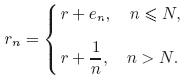
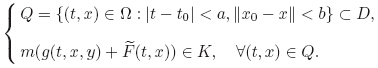 in the sense of the approximate selection theorem
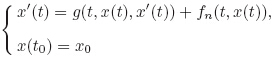
1.12.1 in Ref. [52]. Then,we can see that fn is also Lipschitzean. Let xn : [t0,t0 + T] → Rn be
the solutions of the following problem:
in the sense of the approximate selection theorem
1.12.1 in Ref. [52]. Then,we can see that fn is also Lipschitzean. Let xn : [t0,t0 + T] → Rn be
the solutions of the following problem:
For a subset K ⊂ Rn,the solution for the differential inclusion

Theorem 5 Assume that the graph of K of the set-valued map t ∈ R+ :→ K(t) ⊂ Rn is closed,the map g : (t,x,v) ∈ K × Rn :→ g(t,x,v) ∈ Rn is continuous and affine with respect to v,and the corresponding function F(t,x,y) : Ω × Rn → [0, 1] of the fuzzy map F : Ω → En is upper semicontinuous at (t,x) ∈ Ω. Let α : Rn → [0,1) be a lower semicontinuous function. We posit the following tangential condition:
There exists a constant c > 0 such that
Then,for all x0 ∈ K(0),the following implicit differential inclusion has a viable solution x(·) :

Proof Similar to the construction in Theorem 3,let
 is an upper semicontinuous nonempty compact convex valued map. Set
 is closed,we can easily see that the graph of G is
also closed. Thus,the set-valued map H : (t,x) → G(t,x) ∩ cB has nonempty values by the
tangential condition (TC),and H is also upper semicontinuous (having closed graph and taking
values in compact cB). Thus,H is bounded with the compact convex values and satisfies the
following condition:
is closed,we can easily see that the graph of G is
also closed. Thus,the set-valued map H : (t,x) → G(t,x) ∩ cB has nonempty values by the
tangential condition (TC),and H is also upper semicontinuous (having closed graph and taking
values in compact cB). Thus,H is bounded with the compact convex values and satisfies the
following condition:


Remark 5 By transposing g to the left,we can easily see that (1*) is just a special case of the following IFDI:
In drilling petroleum engineering dynamics,it is crucial to analyze the torque and the drag of the drill-string. In 1986 and 1988,Ho[54, 55] modeled the dynamic performance of the stiff string under the assumption of large deformation,which took the coupling of the axial tension and the torque into consideration. His model is as follows:

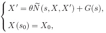
This model is more precise,but it is hard to obtain an analytic solution. One can refer to Ref. [56] for the details and the numerical solutions for this model. For simplicity,we rewrite (3) into the following form:
 < 1. However,because of the uncertainty underground,the dynamic
performance of the drilling system is not that accurate and crisp,which means that the above
differential equation can be modified as follows:
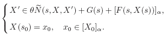
where F(s,X(s)) is a fuzzy map from R+×R2 to E2. Thus,the dynamics of the drilling system
can be represented by an implicit fuzzy initial value problem (IFIVP). To analyze the drilling
performance,it is essential to discuss its solution.
< 1. However,because of the uncertainty underground,the dynamic
performance of the drilling system is not that accurate and crisp,which means that the above
differential equation can be modified as follows:
where F(s,X(s)) is a fuzzy map from R+×R2 to E2. Thus,the dynamics of the drilling system
can be represented by an implicit fuzzy initial value problem (IFIVP). To analyze the drilling
performance,it is essential to discuss its solution.

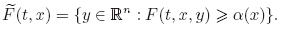
Let α(x) be a constant α ∈ [0, 1]. From the existence theorems presented in this paper,we know that there exists a solution set {X(x0,s)}α,starting from x0 ∈ [x0]α,for the following IFDI:

Examples Suppose that the trajectory of the borehole is r(s). Then,with the rudiments of differential geometry,we can get
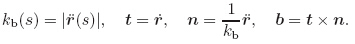
 ,i.e.,
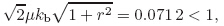
Suppose that F(s,X(s)) = λX(s),which can be regarded as a fuzzy disturbance to the system. Then,(∗) can be interpreted as a family of the IFDIs as follows:


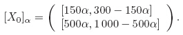
Let
 |
| Fig. 1 Range of {X(s)}0 for IFIVP when λ = 0.5 |
From Fig. 1,we can see that as s increases,X(s) turns out to be crisp. This case comes from the construction of (*),where we simply take F(X(s),s) as λX(s). When we transform this IFIVP into the IFDIs by α-level sets,as [F(X(s),s)]α is singleton,the IFDIs are actually crisp implicit differential equations. Therefore,the perturbation all over the system just comes from the initial values. Moreover,this system is stable under the fuzzy disturbance F. The situation is similar when we alter λ (see Fig. 2).
 |
| Fig. 2 Ranges of {X(s)}0 for IFDIs when λ = 0.5,1.0,and −1.0 |
| [1] | Chen, B. and Liu, X. Reliable control design of fuzzy dynamical systems with time-varying delay. Fuzzy Sets and Systems, 146, 349-374 (2000) |
| [2] | Bede, B., Rudas, I. J., and Bencsik, A. L. First order linear fuzzy differential equations under generalized differentiability. Information Sciences, 177, 1648-1662 (2007) |
| [3] | Puri, M. and Ralescu, D. Differential and fuzzy functions. Journal of Mathematical Analysis and Applications, 91, 552-558 (1983) |
| [4] | Kaleva, O. Fuzzy differential equations. Fuzzy Sets and Systems, 24, 301-317 (1987) |
| [5] | Kaleva, O. The Cauchy problem for fuzzy differential equations. Fuzzy Sets and Systems, 35, 389-396 (1990) |
| [6] | Seikkala, S. On the fuzzy initial value problem. Fuzzy Sets and Systems, 24, 319-330 (1987) |
| [7] | Wu, C. X., Song, S. J., and Lee, E. S. Approximate solutions, existence and uniqueness of the Cauchy problem of fuzzy differential equations. Journal of Mathematical Analysis and Applications, 202, 629-644 (1996) |
| [8] | Song, S., Guo, L., and Feng, C. Global existence of solutions to fuzzy differential equations. Fuzzy Sets and Systems, 115, 371-376 (2000) |
| [9] | O'Regan, D., Lakshmikantham, V., and Nieto, J. J. Initial and boundary value problems for fuzzy differential equations. Nonlinear Analysis: Theory, Methods and Applications, 54, 405-415 (2003) |
| [10] | Choudary, A. and Donchev, T. On Peano theorem for fuzzy differential equations. Fuzzy Sets and Systems, 177, 93-94 (2011) |
| [11] | Nieto, J. The Cauchy problem for continuous fuzzy differential equation. Fuzzy Sets and Systems, 102, 259-262 (1999) |
| [12] | Kaleva, O. Nonlinear iteration semigroup of fuzzy Cauchy problem. Fuzzy Sets and Systems, 209, 104-110 (2012) |
| [13] | Guo, M. S., Peng, X. Y., and Xu, Y. Q. Oscillation property for fuzzy delay differential equations. Fuzzy Sets and Systems, 200, 25-35 (2012) |
| [14] | Ma, M., Friedman, M., and Kandel, A. Numerical solutions of fuzzy differential equations. Fuzzy Sets and Systems, 105, 133-138 (1999) |
| [15] | Abbasbandy, S. and Viranloo, T. Numerical solutions of fuzzy differential equations by Taylor method. Computaional Methods in Applied Mathematics, 2, 113-124 (2002) |
| [16] | Abbasbandy, S. and Viranloo, T. Numerical solutions of fuzzy differential equations by Runge- Kutta method. Nonlinear Studies, 11, 117-129 (2004) |
| [17] | Omar, A. and Hasan, Y. Numerical solution of fuzzy differential equations and the dependency problem. Applied Mathematics and Computation, 219, 1263-1272 (2012) |
| [18] | Yang, L. F. and Li, G. Q. Fuzzy stochastic variable and variational principle. Applied Mathematics and Mechanics (English Edition), 20(7), 795-800 (1999) DOI 10.1007/BF02454902 |
| [19] | Lü, E. L. and Zhong, Y. M. Mathematic description about random variable with fuzzy density function (RVFDF). Applied Mathematics and Mechanics (English Edition), 21(8), 957-964 (2000) DOI 10.1007/BF02428366 |
| [20] | Ma, J., Chen, J. J., Xu, Y. L., and Jiang, T. Dynamic characteristic analysis of fuzzy-stochastic truss structures based on fuzzy factor method and random factor method. Applied Mathematics and Mechanics (English Edition), 27(6), 823-832 (2006) DOI 10.1007/s10483-006-0613-z |
| [21] | Malinowski, M. T. Some properties of strong solutions to stochastic fuzzy differential equations. Information Sciences, 252, 62-80 (2013) |
| [22] | Malinowski, M. T. Random fuzzy differential equations under generalized Lipschitz condition. Nonlinear Analysis: Real World Applications, 13, 860-881 (2012) |
| [23] | Malinowski, M. T. Itô type stochastic fuzzy differential equations with delay. Systems and Control Letters, 61, 692-701 (2012) |
| [24] | Malinowski, M. T. Existence theorems for solutions to random fuzzy differential equations. Nonlinear Analysis: Theory, Methods and Applications, 73, 1515-1532 (2010) |
| [25] | Malinowski, M. T. Strong solutions to stochastic fuzzy differential equations of Itô type. Mathematical and Computer Modelling, 55, 918-928 (2012) |
| [26] | Malinowski, M. T. Approximation schemes for fuzzy stochastic integral equations. Applied Mathematics and Computation, 219, 11278-11290 (2013) |
| [27] | Diamond, P. Brief note on the variation of constants formula for fuzzy differential equations. Fuzzy Sets and Systems, 129, 65-71 (2002) |
| [28] | Hüllermeier, E. An approach to modeling and simulation of uncertain dynamical systems. International Journal of Uncertainty, Fuzziness and Knowledge-Based Systems, 5, 117-137 (1997) |
| [29] | Lakshmikantham, V., Bhaskar, T. G., and Devi, J. V. Theory of Set Differential Equations in Metric Spaces, Cambridge Scientific Publishers, Cambridge (2006) |
| [30] | Lakshmikantham, V. and Mohapatra, R. N. Theory of Fuzzy Differential Equations and Inclusions, Taylor & Francis, London/New York (2003) |
| [31] | Aubin, J. P. Mutational and Morphological Analysis: Tools for Shape Evolution and Morphogenesis, Birkhäser, Boston (1999) |
| [32] | Aubin, J. P. Viability Theory, Birkhäser, Boston (1991) |
| [33] | Diamond, P. and Watson, P. Regularity of solution sets for differential inclusions quasi-concave in a parameter. Applied Mathematics Letters, 13, 31-35 (2000) |
| [34] | Bede, B. and Gal, S. G. Generalizations of the differentiability of fuzzy-number-valued functions with applications to fuzzy differential equations. Fuzzy Sets and Systems, 151, 581-599 (2005) |
| [35] | Li, J., Zhao, A., and Yan, J. The Cauchy problem of fuzzy differential equations under generalized differentiability. Fuzzy Sets and Systems, 200, 1-24 (2012) |
| [36] | Khastan, A., Nieto, J. J., and Rodríguez-López, R. Variation of constant formula for first order fuzzy differntial equations. Fuzzy Sets and Systems, 177, 20-33 (2011) |
| [37] | Khastan, A. and Nieto, J. J. A boundary value problem for second order fuzzy differential equations. Nonlinear Analysis: Theory, Methods and Applications, 72, 3583-3593 (2010) |
| [38] | Zhang, D. K., Feng, W. L., Zhao, Y. Q., and Qiu, J. Q. Global existence of solutions for fuzzy second-order differential equations under generalized H-differentiability. Computers and Mathematics with Applications, 60, 1548-1556 (2010) |
| [39] | Chen, M. H.,Wu, C. X., Xue, X. P., and Liu, G. Q. On fuzzy boundary value problems. Information Sciences, 178, 1877-1892 (2008) |
| [40] | Chen, M. H., Fu, Y. Q., Xue, X. P., and Wu, C. X. Two-point boundary value problems of undamped uncertain dynamical systems. Fuzzy Sets and Systems, 159, 2077-2089 (2008) |
| [41] | Liu, B. Fuzzy process, hybrid process and uncertain process. Journal of Uncertain Systems, 2, 3-16 (2008) |
| [42] | Qin, Z. and Li, X. Option pricing formula for fuzzy financial market. Journal of Uncertain Systems, 2, 17-21 (2008) |
| [43] | Zhu, Y. Uncertain optimal control with application to a portfolio selection model. Cybernetics and Systems, 41, 535-547 (2010) |
| [44] | Baidosov, V. A. Fuzzy differential inclusions. Journal of Applied Mathematics and Mechanics, 54, 8-13 (1990) |
| [45] | Dordan, O. Modelling fuzzy control problems with toll sets. Set-Valued Analysis, 8, 85-99 (2000) |
| [46] | Zhu, Y. and Rao, L. Differential inclusions for fuzzy maps. Fuzzy Sets and Systems, 112, 257-261 (2000) |
| [47] | Zadeh, L. A. The concept of a linguistic variable and its applications in approximate reasoning. Information Sciences, 8, 199-251 (1975) |
| [48] | Lojasiewicz, S., Plis, A., and Suarez, R. Necessary conditions for nonlinear control system. Journal of Differential Equations, 59, 257-265 (1985) |
| [49] | Yannelis, N. C. and Prabhakar, N. D. Existence of minimal elements and equilibria in linear topological spaces. Journal of Mathematical Economics, 12, 233-245 (1983) |
| [50] | Michael, E. Continuous selections I. Annals of Mathematics, 63, 361-381 (1956) |
| [51] | Aubin, J. P. and Frankowska, H. Set-Value Analysis, Birkhauser, Boston (1990) |
| [52] | Aubin, J. P. and Cellina, A. Differential Inclusions, Springer-Verlag, Berlin (1984) |
| [53] | Aumann, R. J. Integrals of set-valued functions. Journal of Mathematical Analysis and Applications, 12, 1-12 (1965) |
| [54] | Ho, H. S. General formulation of drillstring under large deformation and its use in BHA analysis. The 61st Annual Technical Conference and Exhibition of the Society of Petroleum Engineers, Society of Petroleum Engineers, New Orleans (1986) |
| [55] | Ho, H. S. An improved modeling program for computing the torque and drag in directional and deep wells. The 63rd Annual Technical Conference and Exhibition of the Society of Petroleum Engineers, Society of Petroleum Engineers, Houston (1988) |
| [56] | Min, C., Liu, Q. Y., Zhang, L. H., and Huang, N. J. Solutions of the stiff-string model with an iterative method. Journal of Computational Analysis and Applications, 15, 424-431 (2013) |