1 Introduction

Natural convection in open end cavities has many applications such as concentrated so- lar collector,thermal design of buildings,and cooling of electronic equipment^[1]. Solar cavity receiver is also a possible configuration which is widely used in the solar power systems. Cal- culation of thermal losses is very important,and it affects the performance of a solar cavity receiver system. Among the reported studies for natural convection in open end cavity,Chan and Tien^[2] analyzed the steady-state natural convection in a two-dimensional rectangular open cavity. Isotherms and streamlines were reported by those authors in a shallow open cavity with the aspect ratio of 0.143 for the Rayleigh numbers up to 10⁶,considering Boussinesq approxi- mations. Polat and Bilgen^[3] studied laminar,steady state,natural convection heat transfer in inclined shallow cavities. The wall of the cavity (facing to the opening) was heated by a con- stant heat flux,and the sides perpendicular to the heated side were insulated. The opening was also in contact with a fluid at a constant temperature and pressure. The governing equations of continuity,momentum,and energy were solved by assuming that the Boussinesq approxima- tion is valid. Isotherms and streamlines were discussed,and heat transfer was calculated for the Rayleigh numbers from 10³ to 10¹⁰ and for cavity aspect ratio A = H/L from 1 to 0.125. Hinojosa et al.^[4] presented the results of heat transfer in the presence of both natural convec- tion and thermal radiation in a tilted 2D open cavity. The results were obtained for a Rayleigh number ranging from 10⁴ to 10⁷ and for an inclination angle ranging from 0◦ to 180◦. The results showed that the Nusselt number has an increasing trend with respect to the Rayleigh number,except the convective Nusselt number for the case of θ = 180◦,where it remained almost constant. The convective Nusselt number varies significantly with the inclination angle, while the radiative Nusselt number is insensitive to the orientation of the cavity. Bilgen and Muftuoglu^[5] investigated natural convection heat transfer in an open cavity. A uniform heat flux was applied to the active wall facing the opening. The governing equations were solved by the finite difference-control volume method. The important parameters were: the Rayleigh numbers varying from 10³ to 10⁶,the Prandtl number which is set to 0.7,and the cavity aspect ratio,A=L/H=1. The number of slots varied 2 to 8,and the opening ratio varied from 0.1 to 0.6. Their results confirmed that the Nusselt number is an increasing function of the Rayleigh number,while it is a decreasing function of the number of slots and an increasing function of the opening ratio. There is also an optimum opening ratio at large values of Rayleigh numbers. Nouanegue et al.^[6] investigated conjugate convective heat transfer,conduction,and radiation in open cavities with a uniform heat flux (applied to the surface facing the opening). The finite difference-control volume numerical method was used by those authors. The relevant parame- ters were: the Rayleigh numbers varying from 10⁹ to 10¹²,the Prandtl number Pr = 0.7,the cavity aspect ratio varying from 0.4 to 1,the wall thickness l/H = 0.02−0.08,the conductivity ratio varying from 1 to 50,and the surface emissivity varying from 0 to 1. They showed that the convective and radiative Nusselt numbers are decreasing functions of the wall conductance and increasing functions of the aspect ratio. In addition to the references mentioned above, Mohamad^[7],Khanafer and Vafai^[8],Javam and Armfield^[9],and Boetcher and Sparrow^[10] also studied heat transfer in open cavities via conventional computational fluid dynamics (CFD) methods.

In recent years,the lattice Boltzmann method (LBM) has been developed as an alternative to the conventional CFD methods^{[11, 12, 13, 14, 15]}. It has been widely used to simulate heat and mass transfer and fluid flow in cavities with complex geometries^{[16, 17, 18, 19]}. The reasons for turning to this method are the simplicity of programming,locality of computation,natural parallelism,and easiness in dealing with complex boundaries. In addition,conventional CFD simulations are based on the numerical approximations of the Navier-Stokes (NS) and energy balance equations. The NS equations are second-order partial differential equations with nonlinear advective terms. In contrast,the discrete velocity model from which the lattice Boltzmann equation (LBE) model is derived consists of a set of first-order partial differential equations. Moreover,the LBM totally avoids the nonlinear advective terms,because the advection simply uses the data shifting along discrete directions. Considering the advantages of the LBM,Mohamad et al.^[20] simulated natural convection in an open cavity. In their work,the Rayleigh number and the aspect ratio of the cavity were changed in the range of 10⁴-10⁶ and of 0.5-10,respectively. They also compared their results with a conventional CFD method. They found that the heat transfer rate decreases asymptotically as the aspect ratio increases. The rate of heat transfer may also reach conduction limit for large values of the aspect ratio. Jafari et al.^[21] simulated natural convection in an inclined open end cavity for Rayleigh numbers between 10³ to 10⁵ and aspect ratios of 1−4 and for various angles of rotation via the LBM. Their cavity had insulated horizontal walls,while its west wall was maintained at a constant temperature. The results indicated that increasing the aspect ratio leads to a decrease in the average Nusselt number on the hot wall for all the inclination angles. Kefayati et al.^[22] investigated the lattice Boltzmann simulation of natural convection in an open enclosure filled with water/copper nanofluid. In another work,Kefayati^[23] investigated the effect of a magnetic field on natural convection in an open enclosure filled with water/alumina nanofluid using the LBM.

All of the mentioned studies simulated natural convection in cavities with vertically oriented and heated walls. Zhang et al.^[24] simulated lid-driven flow in a two-dimensional isosceles trape- zoidal cavity via the LBM. Nazari et al.^[25] studied steady incompressible fluid flow patterns inside two-dimensional triangle,trapezoidal,semi-circular,and arc-square cavities with moving boundaries by the LBM. Also,Yan and Zu^[26] and Zhang et al.^[27] proposed the scheme for sim- ulation of the thermal boundary condition on a curved wall. Nazari and Shokri^[28] investigated two-dimensional natural convection heat transfer in semi ellipse cavities by the LBM. Recently, Zhou et al.^{[29, 30]} studied aspect-ratio-dependence of heat transfer in natural convection,and their results revealed that heat transfer of the convective system is nearly independent of the aspect ratio of the cell. In this study,we simulate the natural convection in an open end cavity with a hot inclined wall. The combination of the open end cavity with an inclined hot wall is the main novelty of the present study. The main aim of this study is to investigate the effect of the angle of the hot inclined wall on the flow field and heat transfer via the LBM. The highlights of the current research are as follows:

(i) investigation of the effects of the inclined hot wall;

(ii) investigation of different aspect ratios for different inclination angles;

(iii) presenting the local Nusselt number for an inclined hot wall. This is a crucial matter which has not been investigated completely in the literature. 2 LBM model

The two-dimensional nine-velocity (D2Q9) LBM model,as shown in Fig. 1,has been widely and successfully used to simulate incompressible viscous,thermal flows. In this model,two distribution functions are used,and a distribution function of density is used to obtain the macroscopic velocity and density fields,while to calculate the temperature field,a temperature distribution function must be solved,too.

The LBE of the velocity field can be discretized in the space x and the time t into the following form^[31]:

where f_α(x,t) is a distribution function of density of the αth direction in the space x and the time t,Τ_ν is the dimensionless relaxation of the velocity field,δx and δt are the lattice space and the time step size,respectively,and f_α^eq (x,t) is the equilibrium state and has the following form for the D2Q9 model^[31]: where ω_α is the weighting factor given by and c = In the D2Q9 model,e_α denotes the discrete velocity set,namely, F_α is the force term in each direction and can be defined as^[32] where F can be defined as in which β,g_r,and ΔT are the thermal expansion coefficient,the gravity acceleration,and the temperature difference,respectively. The macroscopic velocity and the macroscopic density can be evaluated as According to the incompressible flow,Ma = |u| /c_s«1,and the Chapman-Enskog expansion,the incompressible governing equations can be derived from the D2Q9 model as where the pressure p satisfies the ideal gas equation of state as p = ρc_s² ,and c_s = is the speed of sound. The kinematic viscosity is defined as

Assume that the viscous heat dissipation in the incompressible flow is negligible. The LBE of the temperature field is^[33]

where T_c is the dimensionless relaxation time for the energy equation,g_α(x,t) is the temperature distribution function of the αth direction in the space x and the time t,and g_α^eq(x,t) is its equilibrium state. The fluid temperature T can be obtained as The macroscopic equation of temperature can be recovered through the Chapman-Enskog expansion^[34] and the diffusivity coefficient λ is defined as In the LBM,both Eqs. (1) and (12) are usually solved in two steps,i.e.,streaming and collision. In the collision step, and in the streaming step, where and represent the post-collision states of the distribution function of density and the distribution of temperature,respectively. 3 Boundary conditions in LBM

One of the significant issues in the LBM is how to carry out the collision and streaming steps at the boundaries. Figure 2 shows the details of the heated wall.

The bottom and top boundaries are thermally insulated,while the inclined wall is heated by means of the constant temperature

and the east boundary is open to the ambient. Therefore,we have three kinds of boundaries: open boundary,inclined wall,and horizontal boundary.

(i) Solid straight wall

The bounce back boundary condition is applied on the straight walls of the cavity (north and south boundaries) for both the temperature and the flow.

(ii) Open boundary

Our enclosure has an east open boundary. In this boundary,the following conditions are used^[14].

For the flow,

where n is the lattice on the boundary,and n−1 is the lattice inside the cavity adjacent to the boundary.

For the temperature,if u < 0,then

and if u > 0,then

For more details,one can refer to Ref. ^[14].

(iii) Inclined wall

In Fig. 3,an inclined wall separates the solid region from the fluid region. The black solid circles denote intersections of the wall with various lattice links (x_w),and the lattice node in the fluid region (x_f) and that in the solid region (x_{b) are denoted as the open circles and the grey solid circles,respectively.}

Obviously,to complete the subsequent streaming step,(x_b,t) and (x_b,t) are needed. The fraction of an intersected link in the fluid region is Δ,

To obtain (x_b,t) based upon the known information in the surrounding fluid nodes,the right-hand side of Eq. (18) is defined as^[35] where and

In the above,Χ is the weight factor, = −e_α,and x_ff = x_f + δt. u_f = u(x_f ,t) is the fluid velocity near the wall. u_w = u(x_w,t) is the velocity of the solid wall. u_bf is the imagi- nary velocity for interpolation. To determine the post collision distribution function (x_b,t), we decompose (x_b,t) into the equilibrium part (x_b,t) and the non-equilibrium part (x_b,t). Then,we can get the post-collision step^[26],

where we have used the following relation: The required parameters in Eqs. (28) and (29) are presented in Table 1. In this table,T_f and T_ff denote the temperatures at x_f and x_ff,respectively. 4 Finite volume method (FVM)

Consider laminar,steady,and two-dimensional heat transfer in an open cavity heated from the inclined wall (east wall). The flow is incompressible,and the thermophysical properties of the fluid are independent of temperature,except the density variation. The boundary conditions of the system shown are u = v = 0 for all solid surfaces. On adiabatic boundaries,= 0 is applied. The boundary conditions at the open side of the cavity are summarized as follows:

The numerical method used to solve the macroscopic governing equations is the FVM along with the SIMPLE algorithm. The dependent variables (pressure,velocities,and temperature) are under-relaxed by factors of 0.7,0.3,and 0.5 for p,u,and T ,respectively. For solving the p-equation,a preconditioned conjugate gradient (PCG) solver is used,and for heat and momentum equations a preconditioned bi-conjugate gradient (PBiCG) solver is used. For gra- dient,divergence,and Laplacian schemes,the linear Gauss,upwind Gauss,and corrected linear Gauss schemes are used,respectively. A uniform grid in the X- and Y-directions is used for all computations. The accuracy control is carried out by the conservation of mass by setting its variation to be less than 10⁻⁶ on the pressure term by setting the variation of residues at 10⁻⁶. In addition,the accuracy of computations is checked using the energy conservation within the system by setting its variation to be less than 10⁻⁶. 5 Results and discussion

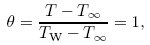
Figure 2 shows the sketch of the problem under consideration. The bottom and top bound- aries are thermally insulated,while the inclined left-wall is heated by means of constant tem- perature (θ=1) and the east boundary is open to ambient. H is the height of the cavity,and γ is the angle of the inclined hot wall. The aspect ratio is defined as A = L/H. For all numerical simulations (by the LBM),201 lattices are used in the Y -direction,and for the X-direction, the number of lattices is equal to 200A. We have further refined the grids by 401 lattices in the Y-direction,but no significant difference in the predicted results is noticed. In the FVM, we use 10 000 and 20 000 cells for the aspect ratios of 1 and 2,respectively. A structured grid generation method is also used in the FVM. The values of the averaged Nusselt number (Nu_ave) at the inclined wall (against the number of grids) are shown in Fig. 4,for both γ=60,80 in the cases of A = 1,2. This figure shows that the obtained numerical results are independent of the number of grids used in the simulations.

Also,to obtain a correct convergence of the numerical simulation,the averaged Nusselt number is plotted against the number of iterations,for different values of γ and the Rayleigh number. The computation is continued to achieve a constant trend (as shown in Fig. 5). In other words,the results are assumed to be converged,when the sum of the averaged Nusselt number approaches a constant value.

We validate our numerical results by comparing with the available results in the literature. Then,the effects of the Rayleigh numbers,the inclined angle,and the aspect ratio are thoroughly studied. The local Nusselt number along the hot surface of enclosure is defined as

where n is the normal direction to the east boundary. The averaged Nusselt number in the physical domain can be expressed as follows: where the integration can be calculated along with the arbitrary vertical line between two isolated boundaries. In other words,in the steady-state condition,the total amount of energy passes through the vertical lines remains constant. Therefore,it is better to calculate Eq. (32) along with an arbitrary vertical line in the computational domain.

In the lattice scale,after some manipulations,one can obtain the following relation for the averaged Nusselt number:

In the LBM,the lattice size (dx_LBM) is equal to one. The summation in the above formula can be done over each vertical line in the computational domain. For γ = 90◦ and A = 1,the cavity is an open square cavity. In this case,we can use the equations of the inclined wall with Δ = 0 as presented in Eq. (23). Accordingly,in order to check the accuracy of our model,the average Nusselt number at the hot wall for γ = 90◦ is calculated and compared with the predictions of Mohamad^[7] and Mohamad et al.^[20]. In these references,the authors used both the FVM and the LBM for a square cavity. This comparison is presented in Table 2. Mohamad et al.^[20] used the D2Q9 configuration to solve the velocity field and the two-dimensional four-velocity (D2Q4) configuration to solve the temperature filed,and the bounce back boundary condition was used for all solid boundaries in the LBM. An excellent agreement is found between our results and those reported in previous studies.

Figures 6−8 show the streamlines and isotherm contours for the Rayleigh numbers 10⁴,10⁵, and 10⁶,A = 1,and γ= 60◦,70◦ and 80◦,respectively.

It can be seen that,for all these inclined angles,when the Rayleigh number is equal to 10⁴, the flow enters from the lower half portion of the open end and leaves from the upper portion of the open end of the cavities. When the Rayleigh number increases to 10⁵,the buoyancy force increases,and the streamlines are tilted upward to the upper-left corner of the inclined wall. By increasing the Rayleigh number to 10⁶,and thereby,increasing the buoyancy force, different recirculation appears at the upper corner of the inclined wall of the cavities. The isotherm contours show that the flow is stratified at the upper half of the cavity. Moreover, the flow is almost isothermal at the lower half of the cavity. Figure 9 shows the variation of the central location of this recirculation with the inclined angle γ. It can be seen that,for all inclined angles,the recirculation approximately appears at a constant height of cavity.

Also,it can be seen from Figs. 6−8 that with the increase in the Rayleigh number,the temperature contours get more and more shifted toward the hot inclined wall. The averaged Nusselt numbers at the inclined wall for R_a = 10⁵ and 10⁶,γ varying between 60◦ to 85◦,and A = 1 are shown in Table 3 and compared with the averaged Nusselt numbers obtained by the FVM for Ra = 10⁶. It can be seen that,when γ increases,the averaged Nusselt number decreases,and therefore the heat transfer rate decreases. In addition,Fig. 10 shows the local Nusselt number (S^*) at the inclined wall for Ra = 10⁶ and A = 1 in different angles. In this figure,the horizontal axis indicates the dimensionless distance along the inclined wall (from the bottom horizontal wall of the cavity).

It can be seen that,in each angle,the local Nusselt number is maximum at the bottom portion of the inclined wall,and it gradually decreases up to the top section. This trend is meaningfully related to the thickness of thermal boundary layer on the inclined surface. The local Nusselt number in the limit case of γ = 90◦ is also shown in the figure. The calculation of the local Nusselt number at the inclined wall is crucial. Therefore,we use several artificial lines perpendicular to the inclined wall of the cavity. Five equal-space nodes are used in the direction perpendicular to the hot surface for calculation of the temperature gradient,i.e.,Eq. (31). The obtained results show that local Nusselt number decreases by decreasing the value of γ,for S^* > 0.6. It may be related to the increase in the thermal boundary layer thickness at the top section of the inclined wall which is affected by the sharp corner of the cavity at the small angles (γ). The scenario of flow development inside the cavity can be expressed as follows:

At the early time,a recirculation is created inside the cavity due to the buoyancy force. On this condition,the flow inside the cavity have no communication with the ambient. In other words,no flow enters from the outside of the cavity. As time proceeds,the above mentioned recirculation is elongated. Therefore,the communication begins between the internal part of the cavity and the ambient. The time needed to start this communication (with the ambient) depends on the aspect ratio,the Rayleigh number,and the angle of the hot wall. As γ increases and/or Ra decreases,the time needed for communication increases. In order to check the accuracy of the LBM results,the temperature distribution obtained by the LBM is compared with that of the FVM at the cross section of Y= 0.5 for Ra = 10⁶ and A = 1 for different angles of γ. Figure 11 shows this comparison. It can be seen that the results of the LBM have good agreement with the results of the FVM.

Figure 12 shows the streamlines and the isotherm contours for Ra = 10⁶,A = 2,and γ = 60◦,70◦,and 80◦. Similar to the case of A = 1,the isotherm contours show that the flow stratification occurs at the upper half of the cavity. Strictly speaking,the flow is almost isothermal at the lower half of this cavity. The streamlines are also tilted upward at the upper corner due to the strong buoyancy force. A recirculation is formed at this corner (see the upper corner of the closed end of the cavity). For this aspect ratio,A = 2,by increasing the hydraulic resistance and the shear stress due to longer horizontal boundaries,the temperature gradient (inside the cavity) remains almost constant along the cavity.

By increasing the aspect ratio,the heat transfer rate (nominated by the Nusselt number) is expected to reach the asymptotically conduction limit. The averaged Nusselt numbers at the inclined wall for Ra = 10⁶, γ between 60◦ to 85◦,and A = 2 are shown in Table 4 and compared with the average Nusselt numbers obtained by the FVM. It can be seen that,when A = 2,the average Nusselt number is lower than that when A = 1 for all inclined angles. Also, the variation of the local Nusselt number at the inclined wall for Ra = 10⁶ and A = 2 is shown in Fig. 13. Similar to A = 1,the maximum local Nusselt number occurs at the bottom portion of the inclined wall.

6 Conclusions

In this paper,the flow field and the temperature distribution for natural convection in open end cavities with inclined walls are studied by the LBM. The main focus of the present paper is to investigate the effects of Ra,the inclined wall angle of the cavity,and the aspect ratio on the flow field,the temperature distribution,and the averaged Nusselt number. The results obtained by the LBM are compared with the FVM,and it can be seen that the LBM results have good agreement with the results obtained by the FVM. The result shows that in all inclined wall angles,when the Rayleigh number increases,the buoyancy force increases,and finally recirculation appears at the upper corner of the cavities. The center of this recirculation emerges at a constant height of the open end cavity. Also,for all Rayleigh numbers,the results show that by increasing the angle of the hot inclined wall,the averaged Nusselt number decreases. For a given angle of the inclined wall,the averaged Nusselt number is decreased by increasing the aspect ratio. It can be seen that,for each angle,the local Nusselt number is maximum at the bottom portion of the inclined wall,and it gradually decreases up to the top section due to the thermal boundary layer development. It is noticed that increasing the aspect ratio decreases the rate of heat transfer and asymptotically approaches the conduction limit.