 2015, Vol. 36
Shanghai University
Article Information
- Zhijie SHI, Yuesheng WANG, Chuanzeng ZHANG. 2015.
- Band structure calculations of in-plane waves in two-dimensional phononic crystals based on generalized multipole technique
- Appl. Math. Mech. -Engl. Ed., 36(5): 557-580
- http://dx.doi.org/10.1007/s10483-015-1938-7
Article History
- Received 2014-08-24;
- in final form 2014-10-08


2. Department of Civil Engineering, University of Siegen, Siegen D-57068, Germany
There is a steady growing interest in both experimental and theoretical investigations on the propagation of elastic/acoustic waves in phononic crystals in the last decades because of their remarkable features[1, 2, 3, 4, 5, 6, 7, 8, 9] . The most interesting and important aspect of these features is that such artificial composites can exhibit elastic/acoustic wave bandgaps, in which elastic and acoustic waves are all forbidden regardless of the polarization and propagation direction of the elastic/acoustic waves. This behavior leads to many interesting physical properties and potential applications. The existence of elastic/acoustic bandgaps is significant for better understanding the propagation properties of elastic and acoustic waves in composite media[10, 11], aswellas various innovative applications such as acoustic filters, ultrasonic silent blocks, and acoustic mirrors. Therefore, one key problem in this research field is to compute the band structures (i.e., dispersion curves) and search for the so-called complete phononic bandgaps. Up to now, several numerical methods have been proposed in literature. Roughly speaking, these methods may be divided into two main categories: eigenfunction expansion methods (meshless methods) and domain/boundary discretization methods (domain or boundary methods). The former category includes the plane-wave expansion (PWE) method[1, 2, 12, 13], the wavelet method[8, 9], the multiple scattering theory (MST) method[14, 15], the Dirichlte-to-Neumann map (DtN-map) method[16, 17, 18], etc. The latter class includes the finite element method (FEM)[19, 20], the lumpedmass method (LMM)[21], the boundary element method (BEM)[22, 23], the finite difference time domain (FDTD) method[24], the spectral element method[25, 26], etc. Each of these methods has its own advantages and disadvantages. For example, the widely used PWE method, the wavelet method, and the FDTD method cannot handle the fluid-solid interface conditions properly. The MST and DtN-map methods are generally convenient, and have much small system matrices for almost all cases including the large acoustic mismatch case. However, these two methods are only suitable for circular and spherical inclusions. The BEM involves singular integrals and may miss some roots (eigenfrequencies)[22]. The FEM is convenient for complex phononic systems with arbitrarily shaped inclusions, but the boundary conditions on the fluid-solid interaction interface are weakened[20], and generally need a large number of elements.
Recently, the present authors have proposed a new numerical strategy to calculate the phononic band structures based on the generalized multipole technique (GMT)[27]. However, only scalar wave propagation in two-dimensional (2D) phononic crystals was investigated[27]. In this paper, the GMT is extended to calculate the band structures of in-plane waves in 2D phononic crystals which are composed of arbitrarily shaped solid or fluid cylinders (including vacuum holes) embedded in a solid matrix medium. According to the basic idea of the GMT[28, 29, 30], the wave fields in the matrix and the inclusion in one representative unit-cell are expanded by using the fundamental solutions with multiple origins. This makes it possible to analyze the phononic crystals with non-circular inclusions. An extra monopole source is introduced which acts as the external excitation. By varying the frequency of the excitation, the eigenvalues can be localized as the extreme points of an appropriately chosen function. By sweeping the frequency range of interest and the boundary of the irreducible first Brillouin zone (FBZ), the band structures can be obtained. In addition, in order to make the extreme points of the response curve more evident, two regularizing procedures are developed[30]. Depending on the use of different basis functions, the GMT can be divided into two categories: the multiple multipole method (MMP)[27, 28, 29] and the multiple monopole (MMoP) method[27, 30]. The present authors have demonstrated in Ref. [27] that the MMoP method can yield satisfactory results. Therefore, in this paper the MMoP method is also used.
The remainder of this paper is organized as follows. In Section 2, the basic vector wave equations and the boundary conditions in a unit-cell are described. A brief overview of the GMT and the derivation of the proposed method for the computation of bandgaps of the phononic crystals are given in Section 3. Then, some numerical examples are presented and discussed in Section 4 to demonstrate the accuracy and efficiency of the method. Finally, Section 5 concludes the paper. 2 Basic equations and boundary conditions
Consider a 2D phononic crystal which is composed of straight and infinite cylinders (inclusions) forming a square or triangular array with the lattice constant a in a matrix (see Fig. 1). The inclusions may be solid, fluid, or vacuum. The cross-section of the inclusions may be of an arbitrary shape. Γ1-Γ4 (Γ1-Γ6) represent the edges of the square (hexagonal) unit-cell, and Γ0 denotes the interface between the matrix and the inclusion. The subscript indices 0 and 1 are used to distinguish the matrix (Ω0) and the inclusion (Ω1) materials. Time-harmonic mixed plane wave modes propagating in the xy-plane are considered.
The governing equations for time-harmonic waves in isotropic and linear elastic solids can be described by the following vector equations[31]:
where x = (x, y) ∈ R2, j = 0, 1, uj(x) = (ux, j(x), uy, j(x)) is the displacement vector at the position x = (x, y), ω is the angular frequency, λj , μj , ρj are the Lamé constant, the shear modulus, and the mass density in Ω0 (j=0) and Ω1 (j=1), respectively, and
 is
the Laplace operator. For convenience, we introduce the Lamé potentials φj and ψj such that
Then, the stress-potential relations are given by
In terms of these potentials, the wave equation (1) is reduced to the following scalar Helmholtz
equation:
where kl, j = ω/vl, j and tt, j = ω/vt, j are the wave numbers of the longitudinal and transverse
waves with vl, j = √ (λj + 2μj)/ρj and vt, j = √ μj/ρj being the velocities of the longitudinal
and transverse waves, respectively.
is
the Laplace operator. For convenience, we introduce the Lamé potentials φj and ψj such that
Then, the stress-potential relations are given by
In terms of these potentials, the wave equation (1) is reduced to the following scalar Helmholtz
equation:
where kl, j = ω/vl, j and tt, j = ω/vt, j are the wave numbers of the longitudinal and transverse
waves with vl, j = √ (λj + 2μj)/ρj and vt, j = √ μj/ρj being the velocities of the longitudinal
and transverse waves, respectively.


 |
Fig. 1 Structures of square lattice (a) and triangular lattice (d) with arbitrary cylindrical inclusions and distribution of sources for matrix ((b) and (e)) and for inclusion (c) (× stands for monopole
sources for matrix,  for monopole sources for inclusion, and for monopole sources for inclusion, and  for external excitation source) for external excitation source)
|
Due to the periodicity of the system under consideration, the computation can be restricted to a single unit-cell. On the interface Γ0 between the matrix and the inclusion, the displacement and traction vectors are continuous for the solid/solid system. Thus, we have
where n(x) is the unit normal vector of Γ0, and σj (x) is the stress tensor on Γ0. In addition, the periodicity of the structure implies that the displacements and tractions should satisfy the Bloch theorem (see Appendix A) on the boundaries of the unit-cell as follows: where i = √ -1 , xm = m1e1+m2e2 with m = (m1, m2) ∈ Z2 and e1 and e2 being the primitive translation vectors, and k = (kx, ky) is a real Bloch wave vector belonging to the FBZ.

If the inclusion Ω1 is an ideal fluid, the displacement field of a propagating wave can be described by a displacement potential η1(x), i.e.,
The pressure p1(x) is then determined by where η1(x) satisfies the Helmholtz equation which is similar to (6) in the frequency domain, i.e., where k1 = ω/v1 is the wave number with v1 = √ λ1/ρ1 being the longitudinal wave velocity. In this case, the boundary conditions on the interface Γ0 require the continuity of the normal displacement and the normal traction as well as the zero tangential traction. Therefore, we have In the case of a vacuum cavity, the traction vector vanishes on the cavity surface, i.e., 3 GMT and calculation of band structures


The GMT[32, 33] is a versatile and reliable numerical method for wave scattering problems in composites with arbitrarily shaped inclusions. It relies on a simple idea, namely, the scattered fields in various domains of the considered composite structure are expressed as a superposition of the fields radiated by adequate sources located outside the corresponding domains. These sources have no physical existence (i.e., fictitious sources) and can be multipole sources or monopole sources. The weights of these sources are unknowns to be determined. To obtain these unknowns, over-determined inhomogeneous linear equations are generated and solved by the least-squares method, and the inhomogeneous term of the equations stems from the incident wave field. In this paper, we use the generalized point-matching technique (GPMT), in which more collocation points than necessary are applied, i.e., the number of the collocation points is larger than the number of the sources or unknowns. Then, we can get the optimal weights of the sources. Once the weights of all the sources are obtained, we can express the scattered wave field in any domain.
For obtaining the band structures of a phononic crystal, an eigenvalue problem without the incident wave field has to be generally solved. However, in the present method, it is difficult to obtain a solution from the over-determined homogeneous linear equations. As suggested in Ref. [27] for anti-plane waves, we can introduce an external fictitious excitation that is applied in such a way that all wave modes are thereby excited. This excitation is equivalent to the incident wave field. This concept mimics the measurement of the resonance frequencies, where one always needs an excitation of the resonator and some test points (or ports) at which the signals are measured. By sweeping the frequency of the excitation, the peaks of an appropriately chosen function in the test points can be readily assigned to the resonance frequencies of the different modes, yielding the eigenvalues we are looking for. Next, we give a brief description of the method. For more details, the readers can refer to Refs. [30]-[33].
According to the above mentioned basic idea of the GMT, instead of the homogeneous wave equation (6), we consider the following inhomogeneous wave equation in the matrix domain Ω0 of the unit-cell:
where ƒl, 0(x) and ƒt, 0(x) are the excitation terms induced by the source at the position xex = (xex, yex) with the wave numbers kl, 0 and kt, 0, respectively. The equation in the inclusion domain Ω1 remains unchanged as (6). If we note that φex(x) and ψex(x) are indeed particular solutions corresponding to ƒl, 0(x) and ƒt, 0(x), respectively, the displacement potentials in Ω0 can be expressed according to the GMT as follows: The displacement potentials in Ω1 can be expressed as follows: For the ideal fluid inclusions, the displacement potential η1(x) in Ω1 can be expressed as In (19)-(23), the superscript “approx” denotes the approximation to the actual fields, aj, n, bj, n, and cj, n are understood as the unknown weights of the sources Sj, n which are located outside the corresponding domains, Fφj, n(x) and Fψj, n(x) are the wave fields radiated from the sources Sj, n and satisfy the governing equation (6), and N0 and N1 are the numbers of the sources for the wave fields in the matrix and inclusion, respectively. According to the Vekua theory[29], Fφj, n(x), Fψj, n(x), and Fη1, n(x) form the complete basis of the series (19)-(23). In the MMP method[29, 30, 31, 32, 33, 34, 35], Fφj, n(x), Fψj, n(x), and Fη1, n(x) take the following identical forms: where Fj, ns is the position vector of the nth source Sj, n, and Hm (1) (·) is the Hankel function of the first kind and mth order. In practical calculations, the truncation m ∈ [−M, M] is taken in (24)-(26). In the MMoP method (also known as the method of fundamental solutions[30] and the method of fictitious sources[33]), Fφj, n(x), Fφj, n(x), and Fη1, n(x) take the following simple forms: In this paper, we use the MMoP method, i.e., (27)-(29). The particular solutions φex(x) and ψex(x) take the same forms as (27) and (28)[29], i.e., To determine the unknown weights, the interface conditions ((7)-(8) for the solid/solid system, (14)-(16) for the fluid/solid system, and (17) for the vacuum/solid system) are imposed on a set of collocation points xk(k = 1, 2, · · · , Nc1) on the interface Γ0. In addition, the Bloch boundary conditions (9) and (10) are imposed on another set of collocation points xk(k = 1, 2, ··· , Nc2) on the boundary of the unit-cell. Then, we can get the following matrix equation: where Ar is an over-determined rectangular matrix with the number of the rows larger than that of the columns, the vector a contains the unknowns ((a0, n, b0, n, a1, n, b1, n) for the solid/solid system, (a0, n, b0, n, c1, n) for the fluid/solid system, and (a0, n, b0, n) for the vacuum/solid system), and the vector b stems from the external excitation source. The specific forms of (32) for the square and triangular lattices are listed in Appendix A. Then, we can get an optimal solution (aopt0, bopt0, abopt1, bopt1)T for the solid/solid system, (aopt0, bopt0, cbopt1)T for the fluid/solid system, and (aopt0, bopt0)T for the vacuum/solid system from (32) based on the least-squares method for a given frequency ω and a Bloch wave vector (kx, ky).


Substituting the optimal solutions aopt0and bopt0into (19) and (20) and subsequently into (2), we can define a norm as
where xt1 = (xt1, yt1) denotes the test point randomly distributed in the matrix domain Ω0, and Nt is the number of the test points. For a Bloch vector (kx, ky) given along the boundary of the irreducible FBZ, the maximum values of the searching function ƒ1(ω, kx, ky) will be found when we sweep the frequency range of interest which does not necessarily start from zero. These maximum values correspond to the eigenvalues we are looking for. Sweeping the boundary of the irreducible FBZ, we obtain the band structures.
It is noted that residual errors are inevitable in the least-squares method. According to (3), we can get the residual error vector in the following form:
Then, we can define another searching function as In order to improve the calculation accuracy, we also introduce an alternative searching function as follows: where p ≥ 2 is the order of this searching function. The eigenvalues to be determined are characterized by the minima of the searching function ƒ2 or ƒ3. In this paper, we use the searching function ƒ3 for the solid/solid system and the vacuum/solid system. For the fluid/solid system, the vibration is localized in the fluid inclusion generally, especially for the fluid with a low density. Thus, we substitute the optimal solution copt1 first into (23) and then into (12), and define another norm as where xt1 = (xt1, yt1) denotes the test point randomly distributed in the matrix domain Ω1. However, if the above method is used directly, the response curve of ƒ3 (or ƒ1, ƒ2, ƒ4)


as a function of the frequency ω may have no extreme point[27, 30]. To overcome this difficulty, Reutskiy[30] proposed two regularizing procedures which can mark out the extreme points clearly. The first one is to introduce a damping term in the governing equations (6) and (13). Then instead of (6) and (13), we have
where ε is a small parameter. In this case, the basis functions (27)-(29) should be modified as In the second regularizing procedure, a shift δk between the wave numbers of the external exciting source and the studied mode is introduced, and then we take the particular solutions as follows: These two regularizing techniques are named as the ε-procedure and δ-procedure, respectively[30]. In general, accurate results can be obtained by using any one of the two procedures. However, the latter one is generally used because the calculations of the Hankel functions with a complex argument in the first procedure are computationally demanding. 4 Numerical examples and discussion


In this section, the above described method based on the GMT is used to calculate the band structures for the mixed modes of the in-plane waves in some typical 2D phononic crystals. In order to validate the present method, the results are compared with those of the FEM. 4.1 Solid/solid system
We first check the accuracy and efficiency of the present method by computing the band structures of the periodic systems composed of circular aurum (Au) cylinders and the epoxy matrix in a square or triangular lattice with the filling fraction ƒ = 0.40. The densities and the wave velocities of the component materials are ρ0 = 1 180 kg/m3, vl, 0 = 2 535 m/s, and vt, 0 = 1 157 m/s for the epoxy, and ρ1 = 19 500 kg/m3, vl, 1 = 3 360 m/s, and vt, 0 = 1 239 m/s for Au. The wave impedance ratios of the systems are ρ1vl, 1/(ρ0vl, 0) = 21.9 and ρ1vt, 1/(ρ0vt, 0) = 17.7. It is well known that some other methods, such as the PWE method[34], may yield poor results for the periodic systems with large acoustic mismatch. In the present method, the distribution of the monopole sources for both the square and triangular lattices is shown in Fig. 2.
 |
|
Fig. 2 MMoP models of phononic crystals with circular inclusions (× stands for monopole sources for matrix, stands for monopole sources for inclusion, * stands for test points, stands for
external excitation, and + stands for collocation points) |
For the square lattice as depicted in Fig. 2(a), the radius of the inclusion is r = a√ f/π = 0.36a, the sources inside the inclusion, outside the inclusion, and outside the unit-cell are distributed along circles with the radii r1 = 0.19a, r2 = 0.52a, and r3 = 0.75a, respectively. We choose the numbers of the sources within the inclusion, outside the inclusion, and outside the unit-cell as N1 = 28 , N2 = 32, and N3 = 40, and the numbers of the collocation points on the interface and the boundary of the unit-cell are Nc1 = 36 and Nc2 = 60, respectively. The number of the test points is Nt = 2 unless otherwise stated. In fact this method is not very sensitive to the number of the test points[29, 30]. The position of the external excitation source is set at xex = (0.2a, 0.1a), and the regularizing parameter in the δ-procedure is δω = δka/(2π) = 1.0. For the triangular lattice, we choose r1 = 0.18a, r2 = 0.50a, r3 = 0.70a, N1 = 24, N2 = 30, N3 = 42, Nc1 = 36, Nc2 = 60, xex = (0.2a, 0.1a), and δω = 1.0. The eigenvalues are obtained from the searching function ƒ3.
 |
| Fig. 3 Band structures of in-plane mixed wave modes in 2D phononic crystal consisting of circular Au cylinders in epoxy matrix with filling fraction ƒ = 0.4 (scattered dots and solid lines are from MMoP method and FEM, respectively, and shadowed regions designate complete band-gaps) |
Figure 3 illustrates the band structures calculated by the present method and the FEM. The vertical axis is the normalized frequency ωa/(2πvt, 0), and the horizontal axis represents the edge of the irreducible FBZ. The results of the FEM are obtained by the acoustics module of COMSOL Multiphysics 3.5a. The numbers of the degrees of freedom are 2 960 for the square lattice and 2 082 for the triangular lattice, respectively. Here, we use the “Direct (SPOOLES)” solver to solve the linear system of algebraic equations. The constraint handling method we used is the “Lagrange multipliers” method. The corresponding computational parameters in the MMoP and FEM models are summarized in Table 1. We can see that the results from the two methods are in good agreement, and they are also in good agreement with those from the DtN-map method[16].
 |
From this example, it is demonstrated that the developed MMoP method can compute the band structures of in-plane waves in 2D solid/solid phononic crystals accurately and efficiently. It is noted that the convergence and the accuracy of the method are affected by many factors including the number and the position of the fictitious sources, the number of the collocation points, the regularizing parameter, and the position of the external excitation soured. Next, we discuss the effects of these factors on the convergence and the accuracy of the present method by taking the square lattice as an example. Of course, similar investigations can be done for the triangular lattice. 4.1.1 Effects of monopole sources and collocation points
We first discuss the influence of the monopole sources by computing the eigenfrequency ωe of the fifth band at k = (π/(2a), 0) for the square lattice (see Fig. 3(a)). Figure 4(a) shows the convergence of the computation with the number of the monopole sources when the number of the collocation points is sufficiently large. Fast and good convergence is observed although some response curves exhibit slight oscillations with the amplitude less than 5 before convergence, as shown in Fig. 4(a1). From these figures, we can find that the minimum numbers of the monopole sources are taben as N1 = 22, N2 = 22, and N3 = 30. Here, we fix the position of the sources, but there is still a certain degree of freedom for setting the position of the sources. Generally, the sources should be sufficiently far from the boundaries[30]. Figure 4(b) shows the convergence of the results with the increase of the distance between the sources and the interface when the numbers of the sources are taken as N1 = 32, N2 = 32, and N3 = 40, and the numbers of the collocation points are chosen as Nc1 = 80 and Nc2 = 120. From this figure, we can conclude that the results are convergent when the numbers of the sources and the collocation points are large enough. However, no convergent result can be obtained when the sources are too close to the expanded domain. For example, no convergence is observed when r1 = 0.30a for the sources inside the inclusion (see Fig. 4(b1)). This is because that some numerical dependencies are induced when the distance between the adjacent sources is too small[29]. Similar behaviors are shown in Fig. 4(b2) and 4(b3) for the sources outside the inclusion and outside the unit-cell.
 |
| Fig. 4 Convergence study of computed results with respect to sources and collocation points for circular inclusions in square lattice |
In the previous examples, we assume that the number of the collocation points is large enough in order to guarantee the convergence. Moreover, the number of the collocation points should be kept to a minimum to reduce the computing time. In the following, we discuss the influence of the number of the collocation points when the number and the position of the fictitious sources are fixed. Figures. 4 4(c1) and 4(c2) show the convergence of the computation with the number of the collocation points for fixed sources. The collocation points are uniformly distributed on the interface and the boundary of the unit-cell. We can observe here that the results are convergent with the increasing number of the collocation points. The minimum numbers of the collocation points for the convergence of the computation are Nc1 = 32 and Nc2 = 44. In practical calculations, we can take Nc1 = 36 and Nc2 = 60 in order to guarantee the convergence.
 |
| Fig. 5 Effects of regularizing parameter and external excitation on response curve for circular inclusions in square lattice |
In the proposed method, the regularizing parameter δω plays an important role in making the eigenvalues more prominent. Figure 5(a) presents the influence of this parameter on the response curves for the square lattices. From this figure, it can be seen that the minimum points (values) of the response curves become evident with the increasing regularizing parameter. In general, we take the regularizing parameter in the range of 0.1 ≤ δω ≤ 2.5. Of course, there are other possibilities for regularizing the response curves, for example, double-precision calculations are used, and the number of the collocation points are increasing. However, they will increase the computational effort.
In order to search the eigenvalues, we introduce a fictitious external excitation which is applied in such a way that all wave modes are thereby excited. This concept mimics the measurement of the resonance frequency. This procedure was first introduced in the method of auxiliary sources[36], and later extended to MMP by Moreno et al.[34] and Smajic et al.[35], and to the method of fundamental solutions by Reutskiy[30]. Interestingly, the type and the location of the external excitation have several options. For convenience, we choose the excitation having the same form as the fictitious sources (see (30) and (31)). The effects of the location of the external excitation on the response curves and the convergence are shown in Fig. 5(b). From this figure, we can observe that the convergence is not sensitive to the location of the excitation. However, the excitation should not be located on the high-symmetry points of the unit-cell. Otherwise, some wave modes cannot be excited, leading to the loss of the roots or eigenfrequencies (see Figs. 5(b3) and 5(b6)).
As mentioned before, the present MMoP method is flexible to deal with arbitrarily shaped inclusions. To demonstrate this advantage, we conduct the computation for a square lattice of Au cylinders with a square (see Fig. 6(a)) or elliptical (see Fig. 6(b)) cross-section embedded in the epoxy matrix. For all cases under consideration, the filling ratio is chosen as ƒ = 0.40. In the case of square inclusions, the side-length of the square inclusion is r = a√ƒ = 0.632 5a. The sources inside the inclusion are distributed along a square with the side-length r1 = 0.50a, the sources outside the inclusion are distributed along a circle with the radius r2 = 0.50a, and the sources outside the unit-cell are distributed along a circle with the radius r3 = 0.75a. The numbers of the sources are taken to be N1 = 48, N2 = 52, and N3 = 60, and the numbers of the collocation points to be Nc1 = 80 and Nc2 = 100. The regularizing parameter is chosen as δω = 1.0, and the position of the external excitation source is selected as xex = (0.2a, 0.04a), as shown in Fig. 6(a). In the system with elliptical inclusions, the ratio of the semi-major axis and the semi-minor axis of the inclusion is assumed as b : c = 0.8 : 1.0. The sources inside the elliptical inclusion are distributed along an ellipse with the semi-major and semi-minor axes being b1 = 0.28a and N1 = 0.36a, the sources outside the elliptical inclusion are distributed along an ellipse with the semi-major and semi-minor axes being b2 = 0.40a and c2 = 0.50a, and the sources outside the unit-cell are distributed along a circle with the radius r3 = 0.75a.
 |
|
Fig. 6 MMoP models of phononic crystals in square lattice with non-circular inclusions (×stands
for monopole sources for matrix, stands for monopole sources for inclusion, * stands for
test points, stands for external excitation, and + stands for collocation points) |
We choose the numbers of the sources as N1 = 44, N2 = 52, and N3 = 60, and the numbers of the collocation points as Nc1 = 68 and Nc2 = 96. The regularizing parameter is taken as δω = 1.0, and the position of the external excitation source is xex = (0.2a, 0.1a) (see Fig. 6(b)). It is important to point out that the numbers of the sources and the collocation points are larger than those in the circular inclusion case. The numbers of the degrees of freedom are 2 810 for the square inclusion case and 2 834 for the elliptical inclusion case, resdentudy. The corresponding computational parameters in the MMoP and FEM models are summarized in Table 1. Figure 7 shows the band structures calculated by the MMoP method (scattered dots) and the FEM (solid lines). It can be seen here that the results obtained by the two methods are in good agreement. The investigated examples verify the applicability of the MMoP method for non-circular inclusions, even for the inclusions with sharp corners.
 |
| Fig. 7 Band structures of in-plane mixed wave modes in 2D phononic crystal in square lattice consisting of non-circular Au cylinders in epoxy matrix with filling fraction ƒ =0.4 (scattered dots and solid lines are from MMoP method and FEM, respectively, and shadowed regions designate complete band-gaps) |
In this subsection, we analyze both the square and the triangular lattices of circular cylindrical vacuum cavities in an aluminum (Al) matrix with the filling fraction ƒ = 0.55. The densities and the wave velocities of the Al matrix are ρ0 = 2 697 kg/m3, vl, 0 = 6 410m/s, and vt, 0 = 3 110 m/s, respectively. The MMoP models for this system are shown in Fig. 2 (but without the sources “T” in the inclusion). The interface condition (17) is used. Here, we choose r1 = 0.20a, r3 = 0.80a, N1 = 40, N3 = 56, Nc1 = 40, Nc2 = 96, δω = 1.0, and xex = (0.2a, 0.1a) for the square lattice, and r1 = 0.20a, r3 = 0.75a, N1 = 36, N3 = 48, Nc1 = 42, Nc2 = 90, δω = 1.0, and xex = (0.2a, 0.1a) for the triangular one. The numbers of the degrees of freedom are 1 400 for the square lattice and 1 032 for the triangular lattice, respectively. The solver of the linear system of algebraic equations and the constraint handling method we used in COMSOL Multiphysics for vacuum/solid system are the same as those for the previously investigated solid/solid systems. The corresponding computational parameters in the MMoP method and FEM models are summarized in Table 1. Figure 8 illustrates the band structures calculated by the MMoP method (scattered dots) and the FEM (solid lines). Here again, we can see that the results from the two methods are almost identical, and that these results are also in good agreement with those of the DtN-map method[16] and the BEM[23]. This validates the applicability of the present GMT for vacuum/solid systems.
 |
| Fig. 8 Band structures of in-plane mixed wave modes in 2D phononic crystal consisting of circular vacuum cylinders in Al matrix with filling fraction ƒ = 0.55 (scattered dots and solid lines are from MMoP method and FEM, respectively, and shadowed regions designate the complete band-gaps) For the considered vacuum/solid system, the effects of the model parameters on the convergence and accuracy are similar to those for the solid/solid systems. Thus, we do not repeat the corresponding discussion here. |
As we know, some numerical methods, such as the PWE method and the wavelet method, do not work well for the fluid/solid system[8, 37]. However, the present MMoP method can calculate the band structures of this mixed system by considering the different wave modes in the fluid and solid as well as the proper fluid-solid interface conditions (14)-(16). In this subsection, we first consider the examples in Subsection 4.2 where the circular cavities are filled now with air. The density and the wave velocity of air are ρ1 = 1.21 kg/m3 and v1 = 340 m/s. This system has a very small acoustic impedance ratio ρ1v1/(ρ0vl, 0) = 0.000 023 8. The MMoP models for this system are shown in Fig. 2. Here, we choose r1 = 0.20a, r2 = 0.56a, r3 = 0.80a, N1 = 36, N2 = 26, N3 = 52, Nc1 = 40, Nc2 = 72, δω = 1.0, and xex = (0.2a, 0.1a) for the square lattice, and r1 = 0.20a, r2 = 0.52a, r3 = 0.75a, N1 = 36, N2 = 24, N3 = 48, Nc1 = 40, Nc2 = 72, δω = 1.0, and xex = (0.2a, 0.1a) for the triangular lattice. The numbers of the degrees of freedom are 2 173 for the square lattice and 1 569 for the triangular lattice, respectively. It is noted here that the “Direct (SPOOLES)” solver is used to solve the linear system of algebraic equations. And the used constraint handling method is again the “Lagrange multipliers” method for fluid/solid systems. The corresponding computational parameters in the MMoP and FEM models are summarized in Table 1, and the eigenvalue searching function ƒ4 is used. Figure 9 shows the band structures calculated by the MMoP method (scattered dots) and the FEM (solid lines). From these figures, it can be recognized that the results obtained from the two methods are almost identical. Moreover, these results are also in good agreement with the results of Ref. [20] (see Fig. 4 therein). A distinguishing feature shown in these figures is the appearance of many flat bands. These flat bands, which are completely different from those appearing when the PWE method is used[37] and did not appear in the predicted results by the DtN-map method[16], are physical bands and associated with the localized vibration modes of the air inside the circular cavity[20]. To better understand these localized vibration modes, we enlarge the curve of the searching function ƒ4 in the normalized frequency range [0.05, 0.25] with the corresponding wave vector k = (π/a, π/a) for the square lattice in Fig. 10. From this figure, we can identify that the flat bands correspond to very small peaks (A, C, D, and E). This implies that these localized vibration modes do not affect the wave propagation behavior in the air/Al system.
 |
| Fig. 9 Band structures of in-plane mixed wave modes in 2D phononic crystal consisting of circular air cylinders in Al matrix with filling fraction ƒ = 0.55 (scattered dots and solid lines are from MMoP method and FEM, respectively) |
 |
| Fig. 10 Bragg scattering mode (B) and localized vibration modes (A, C, D, and E) shown by searching function for air/Al system corresponding to red dashed-line box in Fig. 9(a) |
As the second example, we consider a water/iron system. The material properties of the water are ρ1 = 1 025 kg/m3 and v1 = 1 531 m/s, and those of the iron are ρ0 = 7 670 kg/m3, vl, 0 = 6 010 m/s, and vt, 0 = 3 230 m/s. The acoustic impedance ratio of the system is ρ1v1/(ρ0vl, 0) = 0.034 which is much larger than that of the air/Al system. The filling fraction of this system is ƒ = 0.50. We choose the parameters of the computational model in the MMoP method for this system as r1 = 0.20a, r2 = 0.56a, r3 = 0.80a, N1 = 36, N2 = 26, N3 = 52, Nc1 = 40, Nc2 = 72, δω = 1.0, xex = (0.2a, 0.1a). Here, we choose all the same computational parameters as those in the air/Al system, even though the filling ratio is not exactly the same (see Table 1). Here and in the following examples, we use the searching function ƒ3. The computed band structures are shown in Fig. 11, which are in good agreement with those calculated by the MST method[15], the DtN-map method[16], the FEM[20], and the BEM[23]. It can be seen from Fig. 11 that there is no complete band-gap, and that the number of the flat bands is drastically reduced. This is because that the water has a higher density than the air, and its interaction with the solid is much stronger than that of the air. This example verifies the applicability of the MMoP method for fluid/solid systems with a large acoustic impedance ratio. It also shows that all computational parameters in the proposed method are independent of the material properties, but only depend on the geometry of the periodic structures under consideration. This makes it more convenient to deal with periodic systems having various acoustic impedance ratios. In contrast, the number of the degree of freedom in the FEM is increased drastically (see Table 1), which means that the computational cost is higher.
 |
| Fig. 11 Band structures of in-plane mixed wave modes in 2D phononic crystal consisting of circular water cylinders in iron matrix with filling fraction ƒ = 0.50 (scattered dots and solid lines are from MMoP method and FEM, respectively) |
It is noted that the numbers of the sources and collocation points needed in the vacuum/solid or the fluid/solid system are larger than those used in the solid/solid system.
Next, we consider the system of circular mercury (Hg) cylinders in the Al matrix in a square lattice. The density and the wave velocity of Hg are ρ1 = 13 600 kg/m3 and v1 = 1 450 m/s, respectively. This system has a much larger acoustic impedance ratio ρ1v1/(ρ0vl, 0) = 1.14. The filling fraction is ƒ = 0.40. Similar to the water/iron system, we choose

The corresponding computational parameters in the MMoP and FEM models are summarized in Table 1. The results of the MMoP method and FEM are shown in Fig. 12. They are also in good agreement with those calculated by the DtN-map method[16], the FEM[20], and the BEM[23]. No apparent flat bands can be observed here, because Hg is a special fluid with a very high density at the room temperature, and its interaction with the solid is very strong. From Table 1, we can find that the number of the degree of freedom in the FEM for the Hg/Al system is larger than that for the air/Al and water/iron systems.
 |
| Fig. 12 Band structures of in-plane mixed wave modes in 2D phononic crystal consisting of circular mercury cylinders in Al matrix with filling fraction ƒ = 0.40 (scattered dots and solid lines are from MMoP method and FEM, respectively) |
Finally, we consider the Hg/rubber system which has a very large acoustic impedance ratio ρ1v1/(ρ0vl, 0) = 10.776. The material properties of the rubber are ρ0 = 1 000 kg/m3, vl, 0 = 1 830 m/s, and vt, 0 = 500 m/s, and the filling fraction is ƒ = 0.40. The computational parameters are chosen as

 |
| Fig. 13 Band structures of in-plane mixed wave modes in 2D phononic crystal consisting of circular mercury cylinders in rubber matrix with filling fraction ƒ = 0.40 (scattered dots and solid lines are from MMoP method and FEM, respectively) |
In this paper, we present an accurate and efficient numerical method for the band structure calculations of in-plane waves in 2D phononic crystals based on the GMT. The method expands the wave fields using the fundamental solutions with multiple sources, which makes it possible to deal with periodic composite systems containing non-circular inclusions. An additional excitation source is introduced, and thus the original eigenvalue problem is transformed into a response problem. The extreme values of the response curves correspond to the eigenvalues which we search for. Numerical calculations are performed for typical phononic crystal systems with various acoustic impedance ratios. The following conclusions can be drawn from the present numerical results.
(I) The MMoP method based on the GMT can yield accurate results for the band structures of solid/solid, vacuum/solid, and fluid/solid phononic crystals with various acoustic impedance ratios, including the localized vibration modes. They exhibit some advantages such as good stability, fast convergence, and direct computation in an arbitrary frequency range. In this method, the fluid-solid interface conditions are taken into account strictly for periodic systems with fluid inclusions.
(II) All parameters of the computational model in the MMoP method are independent of the material properties for the same type of periodic systems (solid/solid, fluid/solid, or vacuum/solid), but depend on the geometry of the periodic structure under consideration. This fact makes the method more convenient to deal with phononic crystal systems with various acoustic impedance ratios.
(III) An important feature of the MMoP method is that it can handle periodic systems with arbitrarily shaped inclusions, which is difficult for other methods based on the expansions of cylindrical wave functions, such as the MST and DtN-map methods. Appendix A
Application of the Bloch theorem (see (9) and (10)) to the boundary of a unit-cell of the square lattice leads to the following equations:

Combining (7) and (8) with (A1)-(A6) and taking collocation points Nc1 and Nc2 on the interface Γ0 and the external boundary of the unit-cell, respectively, we have
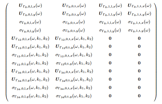

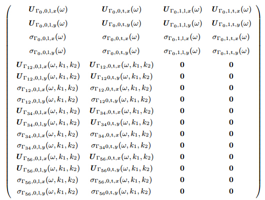
For the triangular lattice, the application of the Bloch theorem to the boundary of a unit-cell leads to similar results which are given by
By combining (7) and (8) with (A8)-(A16) and taking collocation points Nc1 and Nc2 on the interface Γ0 and the boundary of the unit-cell, respectively, the following matrix equation can be obtained:

Similarly, combining (14)-(16) with (A1)-(A6) and taking collocation points Nc1 and Nc2 on the interface Γ0 and the external boundary of the unit-cell, respectively, we can obtain the specific form of (32) for the fluid/solid system in a square lattice as follows:
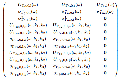

Similarly, for the vacuum/solid system in a square lattice, we can obtain the following equation by combining (17) with (A1)-(A6):
The corresponding equations for the triangular lattices of the fluid/solid and vacuum/solid systems can be obtained similarly but are not given here.
| [1] | Kushwaha, M. S., Halevi, P., Martinez, G., Dobrzynski, L., and Djafarirouhani, B. Acoustic band structure of periodic elastic composites. Physical Review Letters, 71, 2022-2025 (1993) |
| [2] | Kushwaha, M. S. and Halevi, P. Giant acoustic stop bands in two-dimensional periodic arrays of liquid cylinders. Applied Physics Letters, 69, 31-33 (1996) |
| [3] | Yuan, J. H., Lu, Y. Y., and Antoine, X. Modeling photonic crystals by boundary integral equations and Dirichlet-to-Neumann maps. Journal of Computational Physics, 227, 4617-4629 (2008) |
| [4] | Tanaka, Y., Tomoyasu, Y., and Tamura, S. Band structure of acoustic waves in phononic lattices: two-dimensional composites with large acoustic mismatch. Physical Review B, 62, 7387 (2000) |
| [5] | Sainidou, R., Stefanou, N., and Modinos, A. Widening of phononic transmission gaps via Anderson localization. Physical Review Letters, 94, 205503 (2005) |
| [6] | Zhao, Y. C., Zhao, F., and Yuan, L. B. Numerical analysis of acoustic band gaps in twodimensional periodic materials. Journal of Marine Science and Application, 4, 65-69 (2005) |
| [7] | Li, F. L. and Wang,Y. S. Application of Dirichlet-to-Neumann map to calculation of band gaps for scalar waves in two-dimensional phononic crystals. Acta Acustica United with Acustica, 97, 284-290 (2011) |
| [8] | Yan, Z. Z. and Wang, Y. S. Wavelet-based method for calculating elastic band gaps of twodimensional phononic crystals. Physical Review B, 74, 224303 (2006) |
| [9] | Yan, Z. Z., Zhang, C., and Wang, Y. S. Wave propagation and localization in randomly disordered layered composites with local resonances. Wave Motion, 47, 409-420 (2010) |
| [10] | Vasseur, J. O., Deymier, P. A., Beaugeois, M., Pennec, Y., Djafari-Rouhani, B., and Prevost, D. Experimental observation of resonant filtering in a two-dimensional phononic crystal waveguide. Zeitschrift für Kristallographie, 220, 829-835 (2005) |
| [11] | Rupp, C. J., Evgrafov, A., Maute, K., and Dunn, M. L. Design of phononic materials/structures for surface wave devices using topology optimization. Structural and Multidisciplinary Optimization, 34, 111-121 (2007) |
| [12] | Sigalas, M. M. and Economou, E. N. Elastic and acoustic wave band structure. Journal of Sound and Vibration, 158, 377-382 (1992) |
| [13] | Wu, T. T., Huang, Z. G., and Lin, S. Surface and bulk acoustic waves in two-dimensional phononic crystal consisting of materials with general anisotropy. Physical Review B, 69, 094301 (2004) |
| [14] | Kafesaki, M. and Economou, E. N. Multiple scattering theory for 3D periodic acoustic composites. Physical Review B, 60, 11993-12001 (1999) |
| [15] | Mei, J., Liu, Z. Y., Shi, J., and Tian, D. Theory for elastic wave scattering by a two dimensional periodical array of cylinders: an ideal approach for band-structure calculations. Physical Review B, 67, 245107 (2003) |
| [16] | Zhen, N., Li, F. L., Wang, Y. S., and Zhang, C. Bandgap calculation for plane mixed waves in 2D phononic crystals based on Dirichlte-to-Neumann map. Acta Mechanica Sinica, 28, 1143-1153 (2012) |
| [17] | Zhen, N., Wang, Y. S., and Zhang, C. Surface/interface effect on band structures of nanosized phononic crystals. Mechanics Research Communications, 46, 81-89 (2012) |
| [18] | Zhen, N.,Wang, Y. S., and Zhang, C. Bandgap calculation of in-plane waves in nanoscale phononic crystals taking account of surface/interface effects. Physics E, 54, 125-132 (2013) |
| [19] | Axmann, W. and Kuchment, P. An efficient finite element method for computing spectra of photonic and acoustic band-gap materials: I, scalar case. Journal of Computational Physics, 150, 468-481 (1999) |
| [20] | Li, J. B., Wang, Y. S., and Zhang, C. Dispersion relations of a periodic array of fluid-filled holes embedded in an elastic solid. Journal of Computational Acoustics, 20, 1250014 (2012) |
| [21] | Wang, G., Wen, J., Liu, Y., and Wen, X. Lumped-mass method for the study of band structure in two-dimensional phononic crystals. Physical Review B, 69, 184302 (2004) |
| [22] | Li, F. L., Wang, Y. S., Zhang, C., and Yu, G. L. Boundary element method for bandgap calculations of two-dimensional solid phononic crystals. Engineering Analysis with Boundary Elements, 37, 225-235 (2013) |
| [23] | Li, F. L., Wang, Y. S., Zhang, C., and Yu, G. L. Bandgap calculations of two-dimensional solidfluid phononic crystals with the boundary element method. Wave Motion, 50, 525-541 (2013) |
| [24] | Sigalas, M. M. and García, N. Importance of coupling between longitudinal and transverse components for the creation of acoustic band gaps: the aluminum in mercury case. Applied Physics Letters, 76, 2307-2309 (2000) |
| [25] | Wu, Z. J., Wang, Y. Z., and Li, F. M. Analysis on band gap properties of periodic structures of bar system using the spectral element method. Waves in Random and Complex Media, 23, 349-372 (2013) |
| [26] | Wu, Z. J., Li, F. M., andWang, Y. Z. Study on vibration characteristics in periodic plate structures using the spectral element method. Acta Mechanica, 224, 1089-1101 (2013) |
| [27] | Shi, Z. J., Wang, Y. S., and Zhang, C. Z. Band structure calculation of scalar waves in twodimensional phononic crystals based on generalized multipole technique. Applied Mathematics and Mechanics (English Edition), 34, 1123-1144 (2013) DOI 10.1007/s10483-013-1732-6 |
| [28] | Leviatan, Y. and Boag, A. Analysis of electromagnetic scattering from dielectric cylinders using a multifilament current model. IEEE Transactions on Antennas and Propagation, 35, 1119-1127 (1987) |
| [29] | Hafner, C. The Generalized Multipole Technique for Computational Electromagnetics, Artech House, Boston, 157-266 (1990) |
| [30] | Reutskiy, S. Y. The method of fundamental solutions for Helmholtz eigenvalue problems in simply and multiply connected domains. Engineering Analysis with Boundary Elements, 30, 150-159 (2006) |
| [31] | Pao, Y. H. and Mao, C. C. Diffraction of Elastic Waves and Dynamic Stress Concentration, Adam Hilger, U.K. (1973) |
| [32] | Hafner, C. Post-Modern Electromagnetics: Using Intelligent Maxwell Solvers, John Wiley and Sons, New York (1999) |
| [33] | Tayeb, G. and Enoch, S. Combined fictious sources-scattering-matrix method. Journal of the Optical Society of America A, 21, 1417-1423 (2004) |
| [34] | Moreno, E., Erni, D., and Hafner, C. Band structure computations of metallic photonic crystals with the multiple multipole method. Physical Review B, 65, 155120 (2002) |
| [35] | Smajic, J., Hafner, C., and Erni, D. Automatic calculation of band diagrams of photonic crystals using the multiple multipole method. Applied Computational Electromagnetics Society Journal, 18, 172-180 (2003) |
| [36] | Bogdanov, E. G., Karkashadze, D. D., and Zaridze, R. S. The method of auxiliary sources in electromagnetic scattering problems. Generalized Multipole Techniques for Electromagnetic and Light Scattering (ed. Wriedt, T.), Elsevier, Amsterdam, 143-172 (1999) |