1 Introduction

The pipelines for conveying fluids,which have been studied extensively in the past few decades ^{[1, 2]} ,are widely used in various industrial sectors,such as the stream generators,nuclear reactors,and chemical and petrochemical industries. Certain nonlinear dynamics behaviors, such as parametric,external,and internal resonances,as discussed in Refs.^[3]-^[7],can have catastrophic effects on the safety and the functions of these pipelines and the environment. Thus,the proper design of the pipelines and their control to prevent such catastrophic events is extremely important and requires an in-depth understanding of the above mentioned nonlinear dynamic behaviors.

From the viewpoint of nonlinear dynamics,the internal resonance of a pipe can be induced by the natural frequencies of the vibration modes when the ratios of such natural frequencies and the velocity of the fluid reach to certain values. The parameter excited resonance can be induced by the internal turbulence of the flow. Xu and Yang ^{[8, 9]} have investigated the mechanism of the internal resonances between the vibration modes of a pipeline induced by the flow velocity. Their studies revealed that (i) the internal resonance occurs when the natural frequency ratio between the second and first vibration modes reaches to 3:1,and (ii) the periodic motion becomes unstable near the critical fluid velocity by jumping or flutter nonlinear dynamics behaviors. Researchers ^{[7, 8, 9, 10]} have studied the internal resonance combined with the external resonance for the supercritical velocity regime and obtained the relationship of the amplitudes for the two modes. The jumping,hysteresis,saturation,and other complex dynamics behaviors were also presented and discussed.

The parametric and the internal resonances of pipelines conveying fluids are also accom- panied by many complicated nonlinear dynamics behaviors such as flutter,bifurcation,and chaos ^{[11, 12, 13, 14, 15, 16, 17]} . Panda and Kar ^{[4, 5]} investigated the stability and the bifurcation of a pipe un- dergoing the combination of parametric and internal resonances. The periodic,quasi-periodic and chaotic responses have all been observed in their system. In addition,the post diver- gence behaviors including supercritical and subcritical pitchfork bifurcations of extensible fluid- conveying pipes supported at both ends were studied by Modarres-Sadeghi and Paidoussis ^[18] . Jin and Zou ^[19] investigated the local bifurcation of the pipes with the motion-limiting con- straints and linear spring support,and they proved the existence of the quasi-periodic motion and revealed the route to chaos through the breakups of the quasi-period torus surface. Nikolic and Rajkovic ^[20] discussed the influence of the gravitational force,curvature,and vertical elastic support on the bifurcation solutions.

Most above-mentioned analyses have been based on the single-,two- or multi-mode approx- imation of the solutions ^{[3, 4, 5, 7, 10, 11, 12, 16, 18]} . Two- or higher than two-mode approximations have a higher accuracy of the solution for the pipe internal resonance compared with the single-mode only approximation ^[11] . However,multi-mode approximations make the analysis complex,te- dious,and unfeasible for the theoretical analysis. Moreover,it has been discussed in Ref.^[21] that the single-mode approximation of the solution is adequate to capture the dynamic features, to determine the acceptable limits of the pipe vibration and the natural frequencies,which is the foundation of the design criteria for the acceptable level of machinery vibration. Results of Ref.^[12] have demonstrated that both the single- and two-mode approximations essentially give the similar qualitative behavior for the parametric vibration of the pipe under study. Moreover, single-mode approximations may lead to solutions revealing fundamental properties of the pipe system,which is not feasible using the two-mode or higher-mode solution approximations. Our current concern is the vibration induced by the thermal load of the pipes. In many pipeline applications,such as the stream generator,and chemical and petrochemical industries, the fluid is normally transported heatedly through the pipes,and the velocity of the internal fluid often has a harmonic component ^{[22, 23]} . In this process,the effects of the thermal loads on the thermo-elastic relationships of pipe materials and on the nonlinear dynamics behaviors of the pipe have become important and challenging. Although some literatures have focused on the pipe or the container dynamics conveying heated fluids using the cylindrical shell model ^{[23, 24]} , to the best of our knowledge,there is still a lack of systematic exploration on the thermal load effects on the stability and the bifurcation of long and thin pipes ^[25] . Therefore,the objectives of the present work are (i) to analyze the stability and the bifurcation of the pipes conveying fluctuant flow under thermal loads,(ii) to develop a mathematical model governing a simply supported pipe conveying the heated fluid,(iii) to reveal the relationship between the thermal field parameter and the dynamic behaviors of the pipe,and (iv) to give valuable information for the design of the pipeline and the controllers to prevent the structural instability.

The paper is organized as follows. In Section 2,the dynamic equations of the pipe under thermal loads are developed based on the Hamilton principle. The Galerkin method is then applied to discretize the partial differential equations into the ordinary differential equations in Section 3. In Section 4,the stability and the local bifurcation of the lateral parametric reso- nance in both unfolding space and physical state space are analyzed,followed by the numerical simulations in Section 5. Finally,the results and discussions are detailed in the physical state space to gain insights into the pipeline dynamics.

2 Equation of motion

In this paper,we consider a vertical pipe with a length L,an internal cross-section area A, a mass per unit length m,and a flexural rigidity EI. The mass per unit length of a conveying fluid M has an axial velocity U varying with time,referring to a Cartesian coordinate system (OXY ). The pipe is assumed as an Euler-Bernoulli beam initially aligned with the X axis, which is in the direction of gravity. The pipe is assumed to oscillate in the XY -plane. The displacements of the pipe along the X-axis andY-axis are denoted by u and v,respectively ^[1] . The strain of the pipe without considering the thermal load influence can be written as follows ^[1] :

where . Two hypotheses are necessary about the thermal field denoted by T. Firstly,the thermal field is stationary,i.e.,the temperature field does not change with time. Secondly,the temperature of the pipe has a uniform distribution along the radial direction but changes only in the axial direction. Thus,the equation of the temperature distribution subject to one-dimension heat exchange ^[26] is with the temperature boundary conditions: T(0) =Tc and T(L) = T_m,where α t is the thermal diffusivity. Therefore,the first order approximated solution to the thermal field under the above boundary conditions may be expressed as T=c₀+c₁(X + u),where c₀ and c₁ are the coefficients of the thermal field,and c₁ is defined as the linear thermal rate along the pipe axial direction. Negative c₁ represents the decreasing temperature of the conveying fluid,and zero and positive c₁ correspond to the isothermal and the increase in the temperature of the conveying processes,respectively. The symbol is defined as the temperature difference in the small element with the length dX,i.e., ΔT =c₁+c₁ u⁽¹⁾ . The non-linear relationship between the stress σ and the temperature change ΔT was given by Ref.^[25]. where a is the coefficient of the thermal expansion,and h is the coefficient of the non-linear relationship between the stress and the temperature. The parameter h is determined by Mur- naghan’s constant and Poisson’s ratio of the material ^[27] . We obtain the non-linear strain- temperature relationship as follows: For the sake of clarity and convenience,d 1 and d₂ are introduced as d₁= ac₁ and . The strain energy of the system is given by where κ is the curvature of the pipe. The parameters Γ₀ and P are externally applied tension and pressure,respectively. For viscoelastic materials,the damping effect should be considered. As a result,the strain energy should be modified by replacing E with . In the above relationship,e is the coefficient of the Kevin-Voigt damping of the material ^[1] . It should also be noted that the effects of the damping on the thermal stress and the thermal strain are neglected. Based on Hamilton’s Principle,we can obtain the general equations of motion. with the boundary conditions where one dot and two dots denote the first and second derivatives with respect to time t, respectively. Introducing the following dimensionless quantities and parameters: (5) and (6) can be non-dimensionalized as In (9) and (10),τ is the dimensionless time,ū and ¯v represent the relative longitudinal and lateral displacements of the pipe,respectively,and Ū is the dimensionless fluid velocity. 3 Galerkin method

(9) and (10) are the partial differential equations,of which the close-form solutions are rarely found. The Galerkin method is an indispensible method to obtain the approximated solutions. Assume that ū(x,τ) and ¯v(x,τ) can be approximated by the single-mode solution or the two-mode solution below:

or In (11),q₁(τ) and q₂(τ) represent the longitudinal and lateral vibration amplitudes of the single-mode solution in the X-direction and the Y-direction,respectively. In (12),q₁₁ and q₁₂ are amplitudes of the longitudinal vibration of the two-mode solution,and q₂₁ and q₂₂ are the counterparts of the lateral vibration. Substituting (11) into (9) and (10),multiplying the resultant equations by sin(πx),applying the integration from 0 to 1,and considering the orthogonal property of trigonometric functions,we arrive at a set of reduced second-order ordinary differential equations in the coordinates (q₁ ,q₂) T as follows: Similar to the single-mode discretization,using (12),we can obtain the reduced ordinary differ- ential equations in the coordinates (q₁₁ ,q₁₂ ,q₂₁ ,q₂₂)^T for the two-mode discretization. Due to the lack of space in the paper,the two-mode approximation is compared with the single-mode one to demonstrate that the single-mode approximation is adequate for the lateral parametric resonance analysis.

Assume that the pulsating velocity of fluid has the following expression:

where . In the above equations,U₀ is the mean fluid velocity,U₁ is the turbulence velocity,and Ω is the fluctuating frequency of the internal pulsating fluid. Substituting (15) into (13) and (14) yields the two equations as follows: where parameters Δ ₁₁ ,Δ ₁₂ ,Δ ₁₃ ,Δ ₁₄ ,Δ₁₅ ,Δ₂₁,Δ₂₂ ,Δ₂₃ ,Δ ₂₄ ,Δ₂₅ ,and Δ₂₆ are shown in Ap-pendix A.

Since the lateral motion has more effects on the pipe dynamics than that of the longitudinal motion,and (16) and (17) are uncoupled,the lateral motion formulated by (17) is discussed exclusively.

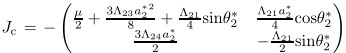
4 Stability and local bifurcation analysis of parametric excited vibration

The system,shown in (17),has positive stiffness when Δ₂₁ is greater than zero and conversely it can have negative stiffness. When the stiffness Δ₂₁ is close to zero for both positive stiffness and negative stiffness,the parametric excited resonance will occur.

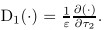
The parameter ω2 is designated as the dimensionless parameter-excited frequency of the first mode lateral vibration . The time scale is changed to τω2 → τ 2 . Normalizing the lateral vibration amplitude q₂ with an initial value r v as ,we obtain the following dimensionless quantities:

For the case of the positive stiffness,the lateral vibration equation (17) can be further non- dimensionalized as follows: For the case of negative stiffness,(17) becomes

In (19) and (20),ε is a small parameter which is used as a book keeping device in subsequent multi-scale analysis. The coefficients in (19) and (20) are shown in Appendix A. Since the positive stiffness and the negative stiffness introduce different nonlinearities,as shown in (19) and (20),they have to be analyzed separately. The analysis procedure and the results for the case of the positive stiffness are discussed in detail,while only the necessary results for the case of negative stiffness are presented due to the similarity of the two analysis procedures.

4.1 Stability and local bifurcation analysis for positive stiffness case

Introducing the tuning parameter,σ₂ ,which describes the difference between Ω₂ and 2_ω2, we consider the parametric resonance when Ω₂ ≈ 2_ω2. When ω₂ = 1,and Ω₂ = 2 + εσ₂ ,for (19),the parameter excited resonance will occur according to Ref.^[28]. The method of multiple scales is used to search for the approximated solution of (19) in terms of the first-order uniform expansion,and the time scale T_n=εⁿτ₂ (n = 0,1) is introduced. The expansion form of q₂ (τ₂) is

The first-order approximated solution to (19) can be expressed as The complex variable modulation equation for the amplitude and the phase can be obtained ^[5] as where Substituting 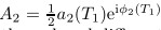into (23) and separating the real part and the imaginary part,we obtain the reduced differential equations of the amplitude and the phase as follows: where θ₂ = σ₂T₁_2φ₂.

(24) and (25) may have the nontrivial solution,{(a₂,θ₂ )|a₂ ≠ 0,or θ₂ ≠ 0},and the trivial solution (0,0). To determine the stability of the nontrivial solution (a₂,θ₂ ) = (a₂^* ,θ₂^*),we assume a₂=a₂^*+ Δa₂ and θ₂ = θ₂^* + Δθ₂ ,where Δaa₂ and Δθ₂ are the small perturbations. Substituting the above expression for a₂ and θ₂ into (24) and (25) yields the following ordinary differential equation for variables (Δa₂,Δθ₂)^T:

where is the Jacobian matrix,and if the real parts of its eigenvalues are all negative,the nontrivial solution a₂ =a₂^*,and θ₂ = θ₂^* is stable. If the real part of one of the eigenvalues is positive,the nontrivial solution a₂ =a₂^* and θ₂ =θ₂^* is unstable. The above method does not work to determine the stability of the trivial solution due to the singularity of the Jacobian matrix. For this case,the Cartesian coordination formulation is utilized ^[5] . Substituting A₂= x₂ + iy₂ into (23),we obtain The solution x₂=0 and y₂ = 0 is the trivial solution of the original system,as shown in (19). The eigenvalues of Jacobian matrix of (27) and (28) determine the stability of the solution x₂ = 0 y₂= 0,and the stability analysis procedure is the same as the nontrivial solution. 4.2 Local bifurcation analysis in unfolding parameter space

Setting the right-hand sides of (24) and (25) to be zero and cancelling θ₂ ,we arrive at the bifurcation equation,

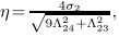
(29) may be further rewritten as (30) is the codimension-2 universal unfolding bifurcation equation with Z-symmetry. The universal unfolding of (30) is given by where δ₁ and δ₂ are the unfolding parameters,η is the bifurcation parameter,and Since the parameters η,ξ,δ₁ ,and δ₂ are relevant because they are all the functions of the physical parameters,bifurcation analysis in the unfold and especially in the physical parameter spaces is necessary. Based on the singularities theory ^[29] ,the various components of the transition set for (31) can be described by the following equations,which are also exhibited in Fig. 2. where H₀ is the hysteresis variety set,B₀ and B₁ are both bifurcation variety sets. The whole unfolding parameter space is divided into eleven regions (a)-(k) by the bifurcation sets B₀ and B₁ ,and the hysteretic set H₀ is depicted in Fig. 1. Figure 2 gives the bifurcation diagrams when the parameters of the system,δ₁ and δ₂ ,are chosen in different regions in Fig. 1. The solid lines plotted in Fig. 2 represent the amplitudes of the stable solutions,and the dashed lines represent the amplitudes of the unstable solutions. The coordinate system of Fig. 2 is shown in Fig. 2(a). The bifurcation diagrams,depicted in Figs.2(a)-2(k),correspond to the unfolding parameter regions of the system when δ₁ and δ₂ are chosen from the regions (a)-(k) as shown in Fig. 1,respectively. Moreover,as shown in Figs.2(f)-2(i),the amplitudes of the stable solutions are zero,which correspond to the unfolding parameter regions (f)-(i) shown in Fig. 1. The amplitudes of zero indicate that the unique solution of (19) is a stable equilibrium point. However,further the distinguishing trivial equilibrium point (0,0) from other non-trivial equilibrium points is needed,which is discussed through simulations in Subsection 5.4.

Some sophisticated dynamics phenomena are also exhibited in Figs.2(a)-2(e),such as jump- ing of the vibration amplitude due to two stable solutions coexisting at certain values of η. Figures 1 and₂ provide comprehensive information about the effects of the parameters on the nature of solutions,such as the types of solutions (equilibrium points or limit cycles) and their stability properties. Such information is significant for the design of the pipeline and the controllers to prevent the structural instability. 4.3 Local bifurcation in physical parameter space

The bifurcation analysis in the unfolding parameter space is impossible to give direct infor-mation about the influence of the thermal rate c₁ on the dynamic behaviors of the system. In order to investigate the influence of the thermal rate c₁ on the stability of the equilibrium point and the limit cycle oscillation (LCO),we map the unfolding parameter space into the physical parameter space. In this work,the assumption of d₂ = 0 is made to simplify the calculation without compromising the accuracy because of the coefficients of the thermal expansion for the pipe material of the steel,a ≈ O(10 _5 ) and . In this study,c₁ is varied,other parameters are kept constant,and the following two equations are solved:

Two solutions for each above equation are obtained and shown in Fig. 3 as c₁ = c_{1_1} and c₁ = c_{1_4} for (35) and c₁ = c_{1_2} and c₁ = c_{1_3} for (36). Let that f₁(c₁ ) = δ₁ (c₁ ),and . The points c_{1_1},c_{1_2},c_{1_3},and c_{1_4} divide the c₁ axis into five regions as shown in Fig. 3. Figure 3 is important in that it connects physical parameters and the unfolding parameters. When the parameter c₁ satisfies {c₁ |c₁≤c_{1 _ 1} } or {c₁ |c₁ ≥c_{1_4} },the system has a unique stable equilibrium point,and the bifurcation diagrams of such an equilibrium point are shown in Figs.2(g) and 2(i). This is because,as {c₁ |c₁≤c_{1 _1} } or {c₁ |c₁ ≥c_{1_4} },δ₁ (c₁ ) > 0 and ξ²δ₁+1/4δ₂²>0. Note that δ₂ is always positive. Referring to Fig. 1,the unfolding parameters, δ₁ and δ₂ ,resulted from the above c₁ are located in the regions (g) and (i),i.e.,δ₁> 0. Further numerical analysis shows that as {c₁ |c₁ ≤c_{1 _ 1} },the pipe dynamic system has the unique equilibrium point of (0,0),while as {c₁ |c₁ ≥ c_{1 _ 4} },the system has a non-zero equilibrium point. The non-zero equilibrium point indicates the existence of static deformation in the pipe, which is of great concern. When the parameter c₁ satisfies {c₁ |c_{1 _ 1} < c₁ ≤c_{1 _ 2} } or {c₁ |c_{1 _ 3}≥ c₁ < c_{1 _ 4} },δ₁ (c₁ ) < 0 and ξ²δ₁+1/4δ₂²>0. The parameters,δ₁ and δ₂ ,are in the regions (j) and (k) in the unfolding parameter space as shown in Fig. 1. The system may have stable periodic solutions for certain values of σ₂ ,and the bifurcation diagrams are shown in Figs.2(j) and₂(k). When c₁ satisfies {c_{1 _ 2} < c₁ < c_{1 _ 3}},δ₁ and δ₂ are in the region (a) of the unfolding parameter space as shown in Fig. 1. The pipe system has stable periodic solutions,and the bifurcation diagram is shown in Fig. 2(a). In summary,when c₁≤ c_{1 _ 1} ,the pipe system has a unique equilibrium point at (0,0). However,when c₁ > c_{1 _ 1},the system may have stable and unstable periodic solutions and equilibrium points upon the tuning parameter σ₂ . Thus,we define the c_{1 _ 1} as the critical thermal rate,denoted by c₁^*. The critical thermal rate c₁^* is an important factor to identify conditions under which the unique equilibrium point at (0,0) exists,which is significant to the parameter selections for the pipe design. When the system stiffness Δ₂₁ < 0 as shown in (17) and Appendix A,the system as shown in (20) has negative stiffness. Since the procedure of the stability and bifurcation analysis is similar to that in the positive stiffness case,only the main result of bifurcation analysis is presented here, . Other parameters ξ, δ₁ ,and δ₂ are all the same as in the positive stiffness case. 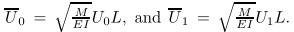5 Numerical simulations

In this section,we first demonstrate the accuracy of the single-mode solution. We then present the results of the bifurcation analysis using such a single-mode solution to reveal (i) the relationship between the amplitude of vibration,a₂ ,and the tuning parameter,σ₂ ,and (ii) the effects of the fluid velocity on the critical thermal rate c₁^*. In simulations,the physical parameters of the pipe lateral vibration dynamic system are chosen from Ref.^[25]. Such parameters are E = 194GPa,I = 5970mm⁴,m = 1.2706kg/m, M = 0.1602kg/m,A = 160mm²,a = 1.1 × 10^-5/◦C,and h = -140E. Throughout the paper unless specifically stated,other parameters used in the simulation are r v = 0.002,e = 0.02, U1 : U0 = 1 : 10,Γ₀=0,P=0,U₀ = 10m/s,L = 5m,and σ₂ = 0. The simulation program was written in MATLAB using the 4th-order Runge-Kutta method. The time step was set as 2 × 10^-5. The MAPLE was used to plot the frequency resonance responses and to calculate the theoretical critical thermal rate c₁^*. 5.1 Comparison between single-mode solution and two-mode solution

In this subsection,we compare the Galerkin single-mode approximated solutions to the two- mode one based on (11) and (12) in Section 3. Two cases are chosen to be presented here, which include c₁ =-2.5 and c₁ = 1.275. The single-mode and two-mode discretizations of longitudinal and lateral vibrations for the above two cases are plotted in Fig. 4 and Fig. 5, respectively. As shown in Fig. 4(a) and Fig. 5(a),the amplitudes of the longitudinal vibration, q₁ and q₁₁ ,are very close,while q₁₂ has a magnitude of 20 percent of the ones of q₁ and q₁₁ . As compared with the lateral vibration,the magnitudes of the longitudinal vibration are extremely low (10^-7 versus 10^-4). Thus,the longitudinal vibration can be neglected. However,consid- ering the lateral vibration,as shown in Fig. 4(b) and Fig. 5(b),the single-mode solution,q₂ ,is reasonable close to the two-mode solution,q₂₁ ,while q₂₂ is approximately zero.

More simulations comparing the single-mode solutions with the two-mode solutions have also been carried out with other values of the parameter c₁ . Similar results have been obtained in that the single-mode solutions approximate the two-mode solutions reasonably well when c₁ < c_{1 _ 2}. Therefore,the first-mode approximated solution of (14) is sufficient to investigate the pipe lateral vibration when c₁ < c_{1_2}

5.2 Relationship between tuning parameter and amplitude of vibration

In this subsection,firstly,we demonstrate the validity of the stability and bifurcation anal- ysis. Secondly,we derive the relationship between the resonance amplitude a₂ and the tuning parameter σ₂ ,which is important for the design of the pipeline systems. Figures 6 and 8 show the results of the stability and bifurcation analyses as discussed in Section 4 using MAPLE. Figures 7 and 9 are the simulated lateral vibration responses with different thermal rates using MATLAB.

When the thermal rate c₁ =1.275,the system has positive stiffness. In the unfolding param- eter space,the system parameters,δ₁ and δ₂ ,are located in the region (j),as shown in Fig. 1, and in the physical parameter space,c₁ is located in {c₁^* < c₁ < c_{1 _ 2} } as shown in Fig. 3. In these regions,the system has periodic solutions. Based on (29)-(34),the frequency response is shown in Fig. 6. Selecting σ₂ = 0 as an example,the time history of q₂ is shown in Fig. 8 with the amplitude of q₂ as 1.06 × 10^-4. Comparing Fig. 6 with Fig. 7,the amplitude of theoretical analysis a₂ as shown in Fig. 6 is 1.16×10^-4,which is consistent with the numerical simulation.

When the thermal rate c₁ = 1.31,the system has negative stiffness. In the unfolding param-eter space,the system parameters are located in the region (j) and in the physical parameter space,c₁ is located in {c_{1 _ 3} < c₁ < c_{1 _ 4} }. The frequency response and the time history of the lateral vibration are shown in Fig. 8 and Fig. 9,respectively. In Fig. 9,the amplitude of q₂ is 3.86×10^-4 when σ₂ = 0. Comparing Fig. 8 with Fig. 9,the amplitude of the theoretical analysis of q₂ as shown in Fig. 8 is 3.92 × 10^-4,which is consistent with the numerical simulation. The consistence among the results from the stability and bifurcation analysis and the simulations for the above two cases of different thermal rates confirm the validity of the bifurcation analysis. We next discuss the relationship between the tuning parameter and the lateral vibration. For the case of the positive stiffness,Fig. 6 depicts that the system will converge to a unique equilibrium point under the condition of the tuning parameter,σ₂ ? _0.19. When _0.19 < σ₂ < 0.19,the system has one stable periodic solution. When σ₂ ? 0.19,the system coexists three solutions including one stable equilibrium point,one stable periodic solution,and one unstable limit cycle. This means that the system will converge to different solutions for different initial values. This result indicates that the jumping phenomenon exists when σ₂ ? 0.19. For the case of the negative stiffness,Fig. 8 shows that the system coexists three solutions,one stable limit cycle,one unstable limit cycle,and one stable equilibrium point. As σ₂ changes from negative to positive,the amplitude of the periodic solution increases gradually.

5.3 Effects of fluid velocity on critical thermal rate

The critical thermal rate c₁^* can provide important conditions under which the attractors of the systems change from the stable equilibrium point (0,0) to the limit cycle. Such information is important for the pipeline design and vibration control. We determine c₁^* using MAPLE through stability and bifurcation analysis by solving (35) as discussed in Section 4. We also determine c₁^* by solving (14) numerically using the Runge-Kutta scheme in MATLAB. The numerical process is briefly described as follows: Firstly,the fluid velocity is fixed,and certain thermal rate of c₁ is selected. We then solve (14) and determine the system attractors as an equilibrium point or a limit cycle by observing the solution trajectories. If the attractor is an equilibrium point,c₁ will be increased,and the simulation will be conducted again. If the attractor is a limit cycle,c₁ will be decreased for simulations. Such a process is iterated to certain values of c₁ ,such that the attractor changes from an equilibrium point to a limit cycle, or vice versa. This specific value,c₁ ,is the critical thermal rate,c₁^*,corresponding to this specific fluid velocity. Figure 10 shows the critical thermal rate for different fluid velocities and pipe lengths. From Fig. 10,we observe that the critical thermal rate c₁^* decreases as the fluid velocity increases regardless of the pipe lengths. Moveover,the critical thermal parameter c₁^* decreases as the length of the pipe increases regardless of the fluid velocity. Figure 10 shows that,although the critical thermal rate c₁^* determined from the theoretical analysis is slightly lower than the one from the numerical analysis,they are overall very close with the maximum error within 21.3 percent. However,the theoretical analysis has the advantages in that it only requires solving the parabolic algebraic equation symbolically once,while the numerical analysis requires solving the ordinary differential equation for a large amount of times,which is time consuming.

5.4 Phase plane trajectories

In this subsection,the findings in the physical parameter space discussed in Subsection 4.3 are demonstrated through simulations. Such findings include (1) when the parameter c₁ satisfies {c₁ |c₁≤ c_{1 _ 1} } or {c₁ |c₁ ≥c_{1 _ 4} },the system converges to the unique stable equilibrium point,and (2) when the parameter c₁ satisfies {c₁ |c_{1 _ 1} < c₁ < c_{1 _ 4} },the system converges to a stable limit cycle at certain σ₂ . We choose L = 5m and U₀ = 10m/s. In this case,c₁^* = 1.262 and c_{1 _ 4} = 1.32 are detected via theoretical analysis in Subsection 4.3. The phase plane trajectories of Eq. (14) via the Runge-Kutta numerical technique are obtained as shown in Figs.11(a)-11(d). On average,iterations are performed 1.585 × 10⁶ time-steps,while the steady state are obtained after 1.0 × 10⁶ time-steps. Figures 11(a)-11(d) are obtained from 1.0 × 10⁶ to 1.585× 10⁶ time-steps. The system converges to the equilibrium point (0,0) as shown in Fig. 11(a) when c₁ = 1.25, which is under the condition c₁ ≥ c₁^* as shown in Fig. 3. The system converges to a limit cycle when c₁ = 1.275 and c₁ = 1.31,which is under the condition,c₁^* < c₁ < c_{1 _ 4} ,as shown in Figs.11(b) and 11(c). The system converges to the non-zero equilibrium point when c₁ =3.0 as shown in Fig. 11(d),which is under the condition c₁ ≥ c_{1 _ 4}. The phase plane trajectory results are consistent with those obtained from the theoretical analysis.

5.5 Chaos of system

Chaos has been detected in this system as shown in Fig. 12. However,when the chaos occur, the velocity of the fluid and the thermal rates are all higher than the critical velocity and thermal rate when the periodical osscilation happens.

6 Conclusions

In this paper,the stability and bifurcation of the pipes under thermal loads have been systematically investigated under the condition that the ratio of the pulsating frequency of the fluid velocity in the axial direction versus the nature frequency of the pipe is approximate,where the parametric resonance will occur. The main results obtained in the paper are as follows: (i) The single-mode approximation of the solution to the above pipe system under thermal loading is adequate to characterize the lateral vibration. (ii) The relationship of the tuning parameter σ₂ and the amplitude of the periodical vibration (or named the frequency response) is obtained. Negative tuning parameters may be beneficial to the stability of the system,because the negative tuning parameter indicates the unique solution such as equilibrium point or the limit cycle,which means that the system will converge to the initial equilibrium state or a periodical vibration on any initial conditions. Higher positive tuning parameters may lead to the jumping phenomena of the system,which means that the system will converge to differential solutions for different initial conditions. (iii) The effects of fluid velocities and pipe lengths on the critical thermal rate have also been investigated. It shows that the critical thermal rate decreases as the fluid velocity increases. The critical thermal rate has the same trend as the pipe length increases. Such findings are important for the pipeline design. (v) Chaos have been detected in this system. However,it only happens when the system is under the condition of a higher fluid velocity and a higher thermal rate. The fluid is often transported heatedly through the pipes in some pipeline industries,and the velocity of the internal fluid has a harmonic component due to the pump and fluid properties. The parametric resonance often occurs,which may have catastrophic effects on the safety and the functions of these pipelines. The investigation of the stability and bifurcation of the pipe system can provide vital information for the design of vibration control for pipe systems conveying heated fluids.