1 Introduction

The theory of shallow water flow is applied often in engineering fields such as coastal ocean engineering and environment engineering because of its importance, and it has been studied extensively^{[1, 2, 3]}. At present, a great number of theoretical models have been proposed for simulating the shallow water flow, such as the Korteweg-de Vries (KdV) equation, the Saint-Venant equation (SVE), and the Boussinesq equation^{[2, 4, 5, 6, 7]}. However, most of the theoretical models that have been proposed are based on the Eulerian method. In the Euler description of shallow water, the flow velocities and the shape of the free surface are treated as unknown variables, and the horizontal velocity is assumed to be independent of the vertical coordinate.

The fluid problem can also be discussed from the Lagrangian perspective^{[1, 3, 8, 9, 10, 11]}. InRef.^[9], Tao applied the Lagrangian method to discuss the sudden starting of a floating body in deep water. In Ref. ^[10], Tao and Shi applied the Lagrangian method to discuss the problem of hydrodynamic pressure on a suddenly starting vessel. In Ref. ^[11], Shi et al. used the Lagrangian method to discuss the nonlinear wave induced by the acceleration cylindrical tank. In the Lagrangian method, the displacements are viewed as unknown variables. One advantage of the Lagrangian method is that the nonlinear boundary condition on the free surface can be exactly satisfied^{[9, 10, 11]}. However, it should be mentioned that in Refs. ^[9]-^[11], the authors obtained the hydrodynamics equations based on Newton’s law rather than the Hamilton variational principle. Undoubtedly, it is important to find a variational principle for the hydrodynamics problem. In the Euler description, it is very hard to find this variational principle. However, it is easy to obtain a Hamilton variational principle by means of the Lagrangian method. Based on the Hamilton variational principle, numerical methods that have been successfully developed and widely applied in structural dynamics, such as the finite element method^[12] and the symplectic method^[13], can be used to simulate the shallow water problem. The symplectic method preserves the symplecticity and energy of the system. Hence, it performs better than the traditional non-symplectic method, especially for problems that require extensive numerical simulation^[13]. Zhong^[8] and Zhong and Chen^[14] used the displacement method, i.e., the Lagrangian method, for the shallow water problem. They treated the displacements as unknown variables and proposed a Hamilton variational principle for the shallow water problem based on the assumption that the horizontal displacement is independent of the vertical coordinate z. According to the Hamilton variational principle, they derived a shallow water equation based on displacement (SWE-D). In Ref. ^[15], the SWE-D was used to analyze the solitary wave problem, and an exact solitary wave solution was obtained. It is convenient to implement the SWE-D numerically because there is only one unknown variable, i.e., the horizontal displacement. However, in the SWE-D, the nonlinear terms related to vertical acceleration are neglected. In this paper, a constrained Hamilton variational principle for the shallow water problem is developed. In the constrained Hamilton variational principle, the incompressible condition is treated as the constraint, and the pressure is seen as the Lagrangian multiplier. According to the constrained Hamilton variational principle, a shallow water equation based on displacement and pressure (SWE-DP) is developed. The SWE-DP contains nonlinear terms related to vertical acceleration that are neglected in the SWE-D.

As the SWE-DP can be deduced from the constrained Hamilton variational principle, it is natural to use the finite element method for space discretization. However, solving the differential algebraic equation (DAE) is inevitable after discreting the unknown variables in space. In Ref. ^[16], a time integration method that could preserve all the constraints was proposed for the DAE. In Ref. ^[17], it was referred to as the Zu-class method. In Ref. ^[18], the Zu-class method was proved to be symplectic. In the Zu-class method, the constraint conditions are satisfied strictly at the integration points, and the phase trajectory is treated as the geodesic one in the state space. The phase trajectory is determined in terms of the least action principle, and the action integral can be approximated by the time finite element method. In this paper, the Zu-class method is used to solve the DAE that results from spatial discretization, and the finite element method is used for the spatial discretization. Hence, we propose a hybrid method for the SWE-DP. The hybrid method combines the finite element method for spatial discretization and the Zu-class method for time integration. The proposed method is symplectic and can preserve the volume numerically. It is especially suitable for simulating the long time evolution of shallow water flow.

2 Basictheory 2.1 Hamilton variational principle for water wave equations

Consider a rectangular tank of two dimensions with two vertical side walls and a horizontal bottom (see Fig. 1). The undisturbed water depth is h, and the length of the tank is L.

Let (x, z) be the location of the particle in the undisturbed water, let u(x, z, t) and w(x, z, t) be the displacements of the particle at time t in x and z, respectively, and let the location of the particle at time t be denoted by (ξ, ζ), in which

The deformation of the water is assumed to be continuous. According to the theory of topology, the particle on the boundary is always on the boundary during the continuous deformation. Hence, the displacements on the boundary are

In terms of the incompressible condition, the determinant of the Jacobi matrix equals one, i.e., Substituting Eq. (1) into Eq. (3) yields where the subscripts denote partial derivatives.

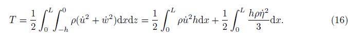
The kinetic energy of the rectangular tank can be expressed as

where $\dot u$ and $\dot w$ are the velocities in x and z, respectively. The potential energy produced by the gravity can be expressed as where ρ is the density, and g is the acceleration of gravity. If treating the incompressible condition as the constraint, we have the following constrained action integral: where p is the Lagrangian multiplier. p is actually the pressure. Calculating the first variation of S gives the water wave equations where $\ddot u$ and $\ddot w$ are the accelerations in x and z, respectively.

2.2 Hamilton variational principle for shallow water equation (SWE)

In the Euler description, the horizontal velocity distribution is assumed to be independent of the vertical coordinate z, because the wave length is much larger than the water depth for the shallow water flow. Here, the displacements are treated as unknown variables. Therefore, we assume that the horizontal displacement is independent of the vertical coordinate z^[8], i.e.,

Substituting Eq. (9) into the third row of Eq. (8) yields which means that the vertical displacement distributes linearly along the vertical coordinate z. At the water bottom, the vertical displacement is zero, and at the free surface, it can be written as Combining Eq. (10) with Eq. (11), we have In terms of Eq. (12), the vertical velocity can be shown as The pressure of the free surface is zero, and that of the water bottom is written as We assume that the pressure distributes linearly along the vertical coordinate z, Substituting Eqs. (9) and (13) into Eq. (5), the kinetic energy can be rewritten as Substituting Eqs. (9), (12), and (15) into Eq. (6), the potential energy can be rewritten as Utilizing Eqs. (9) and (12), the constrained term in the action integral (7) can be written as In terms of Eqs. (16)-(18), the constrained action integral can be rewritten as Calculating the first variation of S gives which is the SWE-DP.

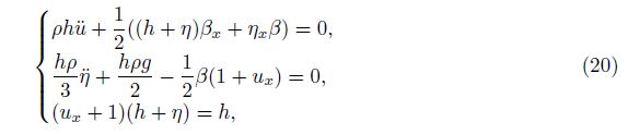
One way to verify the correctness of a new SWE is comparing it with the existing SWEs. In Ref. ^[15], an SWE-D was presented that neglects some nonlinear terms related to the vertical acceleration. Next, we will prove that the SWE-DP (20) can be reduced to the SWE-D. According to the incompressible condition, the vertical displacement of the free surface can be expressed as

Neglecting the nonlinear terms, the acceleration can be written as Substituting Eq. (22) into the second row of Eq. (20), we have Differentiating Eq. (23) with respect to x yields Differentiating Eq. (21) with respect to x yields Substituting Eqs. (21), (23), (24), and (25) into the first row of Eq. (20) and neglecting the third and higher order nonlinear terms of the result yield which is the SWE-D developed in Ref. ^[15].

3 Numerical treatment

It is necessary to develop a numerical method for the SWE-DP. In this section, a hybrid method combining the finite element for spatial discretization and the Zu-class method for time integration is presented in detail.

3.1 Discretization in space

The proposed SWE-DP (20) is derived in terms of the constrained Hamilton variational principle. Hence, it is a natural choice to use the finite element method for spatial discretization.

Let the region [0, L] be divided into N_e basic elements with N_d nodes (see Fig. 2).

On the nth element, the horizontal displacement u(x) is approximated by the linear function, and η(x) and β(x) are treated as constant values, i.e.,

where x_n is the node location in x, Δx_n is the length of the nth element, u_n is the node horizontal displacement, η_n+0.5 is the vertical displacement of the free surface evaluated at the mid-point of the element, and β_n+0.5 is the pressure of the water bottom evaluated at the midpoint of the element. In terms of Eq. (27), the incompressible condition on the nth element can be approximated as Using the lumped mass approach for the kinetic energy, the action integral can be written as in which u and η are the horizontal displacement vector and the vertical displacement vector, respectively. M_u and M_η are the mass matrices corresponding to u and η, respectively. G is the gravity vector, β is the pressure vector, and θ is the vector of volume deformations. M_u, M_η, G, β, and θ can be written as In the integrand of Eq. (29), the summation of the first two terms represents the kinetic energy, the third term represents the potential energy, and the fourth term represents the constrained term. Calculating the first variation of S gives in which With δu₁ = δu_Nd = 0, Eq. (31) gives which constitutes a system of DAEs.

3.2 Zu-class method

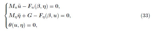
The nonlinear DAE (33) is obtained from the first variation of Eq. (29), which corresponds to a constrained Hamilton system. For the Hamilton system, the symplecticity is a characteristic property. As the symplectic method can preserve the property of symplecticity and the approximate energy necessary for a long time computation, it is often used to simulate the Hamilton dynamical system. However, for the constrained Hamilton system, it is required for a time integration method to preserve not only the symplectic structure of the Hamilton system but also all the constraints. In Ref. ^[16], a method preserving all the constraints was developed by Zhong and Gao. The numerical experiment of the double pendulum presented in Ref. ^[16] showed that this method can preserve energy well. In Ref. ^[17], it was named the Zu-class method. In Ref. ^[18], the Zu-class method was proved to be symplectic. In the Zu-class method, the constraint conditions are satisfied strictly at the integration points, and the phase trajectory is treated as the geodesic one in the state space. The phase trajectory is determined in terms of the least action principle, and the action integral can be approximated by the time finite element method.

In this subsection, the Zu-class method is used to solve the DAE (33). Let the time domain be discretized as

where Δt is the time step. Let the velocities in [t_k, t_k+1] be approximated as where #k = #(t_k), and the displacements can be approximated as

The pressure is approximated to be a constant, i.e.,

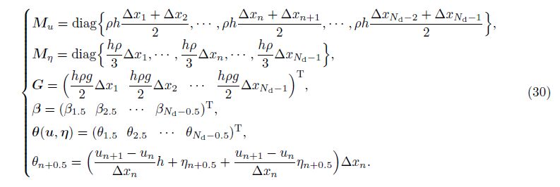
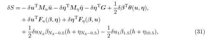
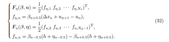
By substituting Eqs. (35)-(37) into Eq. (29), the action integral can be approximated as

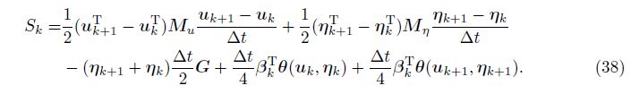
Taking the first variation of the action integral gives

where p_u and p_η are the momentum vectors

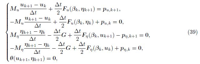
Equation (39) is a system of nonlinear algebraic equations that can be solved by the Newton iteration method. If M_η in Eq. (39) is replaced with M_ηε (ε $ \ll $ 1), Eq. (39) can be used to analyze the shallow water flow ignoring the effect of the vertical acceleration. In this case, the results are in agreement with the SVE solution.

4 Numerical experiments

In this section, the numerical experiments are presented to verify reliability of the SWE-DP proposed in Section 2 and correction of the hybrid numerical method proposed in Section 3 for the SWE-DP. To verify reliability of the SWE-DP, the existing two SWEs, i.e., the SVE and the SWE-D, are adopted. In Subsection 4.1, numerical comparisons with the SVE are given for the case in which the vertical acceleration is neglected. In Subsection 4.2, numerical comparisons with the SWE-D are given for the case in which the vertical acceleration is not overlooked. In Subsection 4.3, numerical experiments are given to verify correctness of the numerical scheme proposed in Section 3.

4.1 Comparison with SVE

Consider a rectangle tank with the length L = 50 m and the depth h = 1 m. The density of water is ρ = 1 000 kg/m³, and the gravitational acceleration is g = 10 m/s². First, we use the SVE for this problem. The initial flow velocity is zero, and the initial free surface is

where ξ = x + u(x, 0). α and A are two parameters controlling the shape of the initial free surface. The smaller α or a is, the flatter the initial free surface is. Here, we set α = 0.3 and A = 0.1 or 0.5. We use the finite difference method with the grid size Δx = 0.1 m and the time step Δt = 0.01 s to solve the SVE.

Then, we use the proposed SWE-DP to simulate this problem. The finite element mesh is uniform with the mesh size Δx = 0.25 m, and the time step for the time integration is Δt = 0.01 s. Because the Zu-class method is used for time integration, the system of nonlinear algebraic equations (Eq. (39)) is involved. We use the Newton iteration method to solve the nonlinear algebraic equations, and the iterative procedure is terminated when the 2-norm of the residual vector is less than 10^-6.

It can be observed that the shape of the initial free surface governed by Eq. (41) is given in the Euler description. In the SWE-DP, the displacement and the pressure are unknown variables. Hence, the initial displacement should be given. In terms of Eq. (41), the initial η(x, 0) is

Substituting Eq. (42) into Eq. (28), we have where N_e is the number of elements, u_n = u(x_n), and In Eq. (43), u₁ = u_Nd = 0. Solving Eq. (43) gives the initial displacement u_n at each node. The initial velocity is zero. Once the initial displacements are obtained, η_n+0.5 can be determined in terms of Eq. (44). To compare the SWE-DP with the SVE, the effect of the vertical acceleration is ignored by setting Mη := 0.001Mη.

Figure 3 shows the free surfaces at different times in the case of α = 0.3 and A = 0.1 computed by the SVE and the proposed SWE-DP. Figure 4 shows the free surfaces at different times in the case of α = 0.3 and A = 0.5 computed by the SVE and the proposed SWE-DP. In Figs. 3-4, good agreement between the SVE solutions and the SWE-DP solutions can be observed.

4.2 Comparison with SWE-D

In this subsection, the numerical comparisons between the proposed SWE-DP and the SWED proposed in Ref. ^[15] are presented with the same rectangle tank used in Subsection 4.1. The initial velocity is zero, and the initial free surface is defined by Eq. (41). The involved parameters are A = 1 and α = 0.1, 0.3. In Ref. ^[15], a method that combined the finite element method with the symplectic time integration method was proposed for the SWE-D. The method is used here to solve the SWE-D, the finite element is uniform with the mesh size Δx = 0.25 m, and the time step for the time integration is Δt = 0.01 s.

The hybrid method proposed in Section 3 is used to solve the SWE-DP. The finite element is uniform with the mesh size Δx = 0.25m. The time step for the Zu-classmethod is Δt = 0.01 s. The involved nonlinear algebraic equations in the Zu-class method will be solved by the Newton iteration method with the residual error 10^-6.

Figure 5 shows the free surfaces at different times in the case of α = 0.1 and A = 1 computed by the SWE-D and the proposed SWE-DP. Figure 6 shows the free surfaces at different times in the case of α = 0.3 and A = 1 computed by the SWE-D and the proposed SWE-DP. In Fig. 5, good agreement between the SWE-D solutions and the SWE-DP solutions can be observed. However, in Fig. 6, slight differences can be observed between the SWE-D solutions and the SWE-DP solutions. The slight differences reflect the differences between the SWE-D and SWEDP. The SWE-D neglects the nonlinear terms associated with the vertical acceleration, which are, however, considered in the SWE-DP. The effects of these nonlinear terms associated with the vertical acceleration are weak in the case of α = 0.1.

4.3 Convergence of proposed numerical method

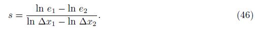
The proposed numerical method combines the finite element method for spatial discretization and the Zu-class method for time integration. Hence, the error of the proposed method depends on two factors, i.e., the mesh size and the time step. The effect of the mesh size on the proposed method is discussed first using different mesh sizes and the same time step. In this case, the numerical error can be expressed as e = CΔx^s, in which C is a constant independent of the mesh size Δx, and s is the order of accuracy associated with the mesh size. Thus, the errors e₁ and e₂ for two different mesh sizes Δx₁ and Δx₂ can be given by

and the order of accuracy can be shown by Five mesh sizes Δx = 1/20 m, 1/40 m, 1/80 m, 1/160 m, and 1/320 m are selected to determine the order of accuracy. The solutions with the mesh size 1/320 m are seen as the reference solution. The time step is Δt = 0.01 s. The other parameters are α = 0.1, 0.3 and A = 0.8. We select nine observation values, i.e., the displacements u(12.5, t), η(12.5, t) and the pressures β(25, t) at different times t = 1 s, 2 s, and 5 s, to test convergence and order of accuracy. The observation values, calculated by the proposed method with different mesh sizes, for α = 0.1 and α = 0.3 are listed in Tables 1 and 2, respectively. By Eq. (46), the order of accuracy associated with the mesh size can be calculated. Nine orders corresponding to the nine observation values are also included in Tables 1 and 2. Table 1 is for the case in which α = 0.1, and Table 2 is for the case in which α = 0.3.

Next, we test the effect of the time step on the accuracy of the proposed method. Let the numerical error be expressed as e = CΔt^l, in which C is a constant independent of the time step Δt, and l is the order of accuracy associated with the time step. For two different time steps Δt₁ and Δt₂, the errors are

and the order of accuracy can be expressed as Five time steps Δt = 0.2 s, 0.1 s, 0.05 s, 0.025 s, and 0.001 s are selected, and the solutions computed by using the smallest time step are seen as the reference solutions. The mesh size is Δx = 0.5 m. The other parameters are α = 0.1, 0.3 and A = 0.8. Nine observation values used for testing the effect of the mesh size on the accuracy of the proposed method are still utilized. The observation values computed by using the proposed method with different time steps for the cases in which α = 0.1 and α = 0.3 are listed in Tables 3 and 4, respectively. By using Eq. (48), the order of accuracy associated with the time step can be computed. Nine orders corresponding to the nine observation values are also included in Tables 3 and 4. Table 3 is for the case in which α = 0.1, and Table 4 is for the case in which α = 0.3.

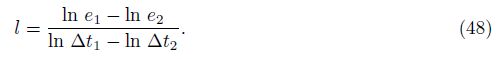
From Tables 1-2, it can be seen that all nine observation values converge to the reference solutions as the mesh size gradually becomes small, and the order of accuracy associated with the mesh size is approximately 2. From Tables 3-4, it can be seen that all nine observation values converge to the reference solutions as the time step gradually becomes small, and the order of accuracy associated with the time step is approximately 2. Hence, it is possible to conclude that the accuracy of the proposed method is second order.

The performance of the long time simulation of the proposed method is further tested by observing the conservation of the numerical energy over time. The total energy of the system is the summation of the kinetic energy and the potential energy. In terms of Eqs. (29)-(30), the numerical energy can be expressed as

The time step and the mesh size are Δt = 0.1 s and Δx = 0.5 m, respectively. The integral interval is [0, 100] s. α = 0.1 and 0.28. A = 0.8. The relative error of the energy is (H(t) - H(0))/H(0).

Figure 7 shows the variations in the relative energy errors versus the time. The dashed line is for α = 0.1, and the solid line is for α = 0.28. From Fig. 7, it can be concluded that using the proposed method for the SWE-DP, the energies are preserved well for a long time.

For the SWEs in the Euler description, it is inconvenient to obtain the motion curve of particles during the oscillation of the water. However, the motion of particles in the water can be conveniently obtained using the proposed SWE-DP, as the displacement and the pressure are treated as unknown variables. Figure 8 shows two motion curves of the same particle in different cases. The particle is located at (12.5, 0) m when the water is not distributed. The two motion curves correspond to the case of α = 0.1 and α = 0.28, respectively. From Fig. 8, a large difference can be observed between the two motion curves. In the case of α = 0.1, the motion curve is not closed, while the motion curve is nearly overlapped in the case of α = 0.28. The motion of the particles in the case of α = 0.28 is of an approximate period, and the water wave propagates like the solitary wave, which can be demonstrated by Fig. 9, in which the evolution of the free surface is shown. From Fig. 9, it can be seen that the free surface approximate periodically changes about 6.5 times within 100 seconds.

5 Conclusions

The constrained Hamilton variational principle for the shallow water flow is developed. Based on the constrained Hamilton variational principle, the SWE-DP is developed. a hybrid numerical method combining the finite element method for spatial discretization and the Zuclass method for time integration is created for the SWE-DP. The correctness of the proposed SWE-DP is verified by numerical comparisons with two existing SWEs, i.e., the SVE and the SWE-D proposed in Refs. ^[8] and ^[15]. The correctness of the hybrid numerical method proposed for the SWE-DP is also verified by the numerical experiments. Moreover, numerical experiments show that the Zu-class method performs well in the simulation of the long time evolution of the shallow water.

In this paper, we only consider shallow water with two dimensions and a horizontal bottom. However, the basic ideas can be expanded to other hydrodynamics problems. Compared with the Eulerian method, it is more convenient to deal with the nonlinear boundary condition on the free surface and to develop the Hamilton variational principle using the Lagrangemethod. Based on the Hamilton variational principle, the numerical methods which have been successfully developed and widely applied in structural dynamics, such as the finite element method^[12] and the symplectic method^[13], can be used to simulate hydrodynamics problems. The symplectic method preserves the symplecticity and energy of the system and, hence, performs better than traditional non-symplectic methods, especially for problems that require numerical simulation for a very long time^[13]. In a word, we believe that the displacement method will play a major role in accurately and efficiently simulating hydrodynamics problems. In our next work, the proposed method will be expanded to shallow water with three dimensions and a sloping bottom.