 2016, Vol. 37
Shanghai University
Article Information
- Wenwen LIU, Jie PENG Keqin ZHU. 2016.
- Finite depth Stokes' first problem of thixotropic fluid
- Appl. Math. Mech. -Engl. Ed., 37(1): 59-74
- http://dx.doi.org/10.1007/s10483-016-2016-9
Article History
- Received Mar. 12, 2015;
- in final form Jun. 15, 2015


Thixotropic fluids are used widely in civil engineering, food, cosmetic, and pharmaceutical industries, and impact every aspect of our lives. As emulsions, suspensions, or polymeric gels, they are very different from each other compositionally, but most of them have one thing in common, i.e., the existence of microstructures. The microstructures are changeable and may comprise a network of flocculated colloidal particles, tangles of polymers, or a spatial arrangement of suspended particles or drops[1]. On one hand, it can be established gradually while the material is at rest (which is called aging or healing). On the other hand, it can be destroyed due to the shear of the materials (which is called rejuvenation or destructuration)[2, 3]. As a result, the effective viscosity of this material can change continuously while the microstructure varies.
Thixotropic fluids have a lot of special characters, such as aging, rejuvenation, and viscosity bifurcation[4]. Up to now, a lot of efforts have been made to explore the rheological property of the material, and several models have been presented[5, 6, 7]. Most of them belong to the structural kinetics model, which was first proposed by Moore[8] in 1959. The structural kinetics model characterizes the local state of the microstructure by a single scalar parameter governed by an appropriate evolution equation. Similar models have also been introduced by Houska[9], Worrall and Tuliani[10], and Dullaert and Mewis[11]. Mewis and Wagner[5] summarized these models in a general form. One of the most popular structural kinetics models in recent investigation was presented by Coussot et al.[2]. The avalanching behavior of start-up flow on slopes can be predicted successfully according to this model[12, 13, 14]. The Coussot model is quite special among the structural kinetics models, because the yield stress is introduced implicitly. In recent studies, Roussel et al.[15] and Coussot et al.[16] suggested that the yield stress fluid can be classified into two classes: the simple yield stress fluid and the thixotropic yield stress fluid. It is shown that the former one can be characterized by the Herschel-Bulkley model, and the Coussot model characterizes the later one quite well in their experiments.
Though a lot of thixotropic models have been developed based on rheological experiments, few studies are concerned with the flow characters of thixotropic fluids in practical situations such as conduit flows[17, 18] and slope flows[12, 13, 14]. Liu and Zhu[13] studied the start-up flow of thixotropic fluids including inertia effects on an inclined plane. The effects of the unsteady term in the Navier-Stokes equations on the start-up process were clarified. McArdle et al.[19] studied Stokes’ second problem of thixotropic fluids, which means a semi-infinite fluid bounded by an oscillating wall. They discussed both fast-adjusting and slowly-adjusting behaviors of thixotropic fluids, and the solutions showed significant difference from the classical solution for the Newtonian fluid. However, the yield behavior was not considered.
Stokes’ first problem, also known as Rayleigh’s problem, is one of the most classical problems of unsteady flow. For the Newtonian fluid with a constant kinematic viscosity ν, an exact solution for the velocity can be derived as
 . When the fluid is bounded by the wall
and a free surface, the problem can be considered as a finite-depth Stokes’ first problem[21]. For
the Newtonian fluid, the exact solution of the velocity profile is
. When the fluid is bounded by the wall
and a free surface, the problem can be considered as a finite-depth Stokes’ first problem[21]. For
the Newtonian fluid, the exact solution of the velocity profile is
In recent years, Stokes’ first problems for a couple of non-Newtonian fluids have been investigated. For example, Jordan et al.[22] examined Stokes’ first problem for the Maxwell fluid using integral transform methods. The exact solution of this problem was clarified compared with former studies[23]. Tan and Masuoka[24, 25] considered Stokes’ first problem for the second-grade fluid and the Oldroyd-B fluid in a porous half space. Qi and Xu[26] extended the constitutive model in this problem to a fractal, or generalized, Oldroyd-B fluid. Most of these studies focused on the flow of visco-elastic fluid. Although simple start flow in heterogeneous simple shear is a common testing case for exploring the materials’ rheological behavior, to the best of the authors’ knowledge, Stokes’ first problem of thixotropic yield stress fluids has not been studied yet. In this study, the Coussot model is adopted to describe the property of thixotropic yield stress fluid. The flow characters and the effects of dimensionless parameters in this problem are discussed.
In the remainder of this paper, we give a brief introduction about the constitutive equation and the governing equation of this problem in Section 2. Then, in Section 3, the results through numerical calculation are discussed, including the velocity profile, the shear stress on the wall, and other flow characters. Finally, conclusions are made in Section 4.
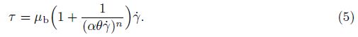
2 Mathematicalmodel 2.1 Rheological modelThe Coussot model is noted as follows[2]:


Here, the first term on the right-side of Eq. (4) represents aging, and the second term represents rejuvenation. τ is the shear stress, $\dot \gamma $ is the shear rate, and λ is the structure parameter. μb describes the basic viscosity of the material in the absence of microstructures (λ = 0). n is the power exponent about the relationship between the effective viscosity and the microstructures. The viscosity bifurcation happens when n > 1[2]. θ is the characteristic time of aging. A bigger θ means a slower aging process. The microstructures can be destroyed by shear, and α indicates the intensity of this destruction procedure. The Coussot model was first proposed to reproduce the physical properties of yield stress fluids[2]. It has some special features, which can be seen clearly from the equilibrium flow curve (EFC). After a fixed shear stress or the shear rate is imposed on it for a long time, the structure parameter tends to be constant, and the flow tends to an equilibrium state. The long term feature of the material is then determined according to the relationship between the shear stress and the shear rate under this condition. According to Eqs. (3) and (4), the EFC of the Coussot model can be determined as follows:
Clearly, it can be reduced to the Bingham model while n = 1. However, as it was pointed out by Coussot et al.[2], the case that n > 1 fits the experimental result better. The EFC of this case is illustrated in Fig. 1. It can be divided into two branches according to the point with the minimal shear stress, which can be regarded as the yield stress.

|
| Fig. 1 EFC of Coussot model and division of yield and unyield regions when μb = 1, αθ = 1, n = 1.2, and implicit yield stress is about 2 |
On the left branch of the EFC, the shear stress decreases with increasing the shear rate, which means that this branch is not stable. Although this behavior is not physically unrealistic as it seems, it has been verified by the experimental results[27, 28]. The shear stress increases normally with increasing the shear rate on the right branch of the EFC. It is then claimed as the stable branch.
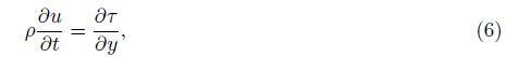
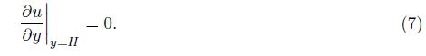
2.2 Governing equationWe consider the finite depth Stokes’ first problem. The thickness of the thixotropic fluid layer is H. The boundary wall suddenly moves in the x-direction with the velocity U0. The velocity component can be written as [u, v] = [u(y, t), 0], in which y is the spanwise coordinate, and t is the time. The continuity equation and the momentum equation in the y-direction can be satisfied automatically, and the momentum equation in the x-direction can be simplified as
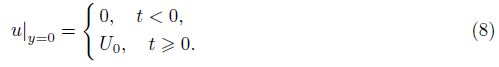
At the initial state, the fluid is assumed to be quiescent with

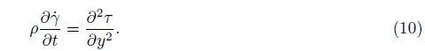
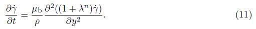
Taking the derivative of y on both sides of Eq. (6), we get an equation related to the shear rate,


Here, Re = ρhU0/μb is the Reynolds number. We = θ/(h/U0) is the Weissenberg number, which defines the ratio of characteristic time between aging and flow. A small We means that microstructures can change rapidly with the local shear stress, which makes the flow tend to the structural equilibrium flow state. On the contrary, a large We makes microstructures hard to change so that the flow tends to the structural frozen state. Rj = αλ0 is defined as the rejuvenation number, which indicates the intensity of the rejuvenation effect. It can be realized as the ratio of the characteristic time of rejuvenation and the characteristic time of aging, because αθλ0 is the reciprocal of the characteristic shear rate and the shear rate with the dimension of t-1. Therefore, the rejuvenation effect is remarkable in the case of small Rj.
The coefficient of flow unsteady term We/Re in Eq. (16a) indicates how fast the flow field can evolve to adapt a new boundary condition or other influencing factors. If We/Re is large, any little change on the right-hand side of Eq. (16a) brings a large ∂$\dot \gamma $/∂t to keep balance of this equation. That means the flow field evolves so fast that it achieves a new steady state instantly. Apparently, the inertial force slows down the velocity evolvement, and the viscous force speeds up the velocity evolvement.
According to the experiments of Roussel et al.[29], for bentonite suspension, θ is on the order of 100 s-102 s, α is on the order of 10-2 s-10-4 s, ρ of the suspension can be replaced by the density of water, and μb is on the order of 10-1 Pa·s. The non-dimensional parameters in a real flow can be estimated accordingly.
2.3 Numerical methodIn the study, the finite difference method is used to simulate the flow. A fourth-order Runge- Kutta scheme is adopted to discretize the time evolution, and a centered difference scheme is adopted to discretize the space direction, i.e., the y-direction. Considering a great velocity gradient which may appear near the wall, we use uneven grid throughout the flow region. Finer grids are applied near the wall. The second-order central difference formula is modified accordingly. When the right-hand side grid is m times larger than the left-hand side one, this formula becomes
It has been mentioned in the previous section that the flow characteristics can be affected directly by We/Re, ReRj, and the initial structure parameter λ0. In this section, two kinds of flow, i.e., the non-yield flow and the yield-like flow, are mainly considered. The effects of We/Re, ReRj, and λ0 are discussed.
3.1 Non-yield flow caseIn this case, the effective viscosity variation throughout the flow field is relatively small. Therefore, the features of the flow cannot be described properly by the concept of yield. In fact, this means that the rejuvenation effect is weak, since it is the only process to make the effective viscosity become uneven.
Actually, the rejuvenation procedure is affected by many factors. When We/Re is relatively large, the flow evolves much faster than the changing of microstructures, and all the thixotropic effects including aging and rejuvenation can be ignored. The velocity profiles are plotted in Fig. 2, where the vertical axis represents the dimensionless velocity u, and the horizontal axis represents the span-wise coordinate y. The walls located at y = 0 and y = 1 indicate the positions of the free surfaces. The solid lines are the velocity profiles of the thixotropic fluid with the nondimensional parameters We/Re = 1, ReRj = 0.01, and λ0 = 10. The dashed lines are the velocity profiles of the Newtonian fluid with a finite depth. It is based on the exact solution shown by Eq. (2). As we can see in Fig. 2, these two curves almost overlap with each other all the time. This means that the characteristic time of flow is much shorter than the characteristic time of aging, i.e., We has large values. The velocity evolvement has already finished before the material shows any thixotropic effects. Besides, we draw the velocity profiles of Newtonian fluid with an infinite depth (the standard Stokes’ first problem) in dashdot lines in Fig. 2. Although the exact solutions of finite depth and infinite depth have different mathematical forms, their velocity profiles do not show noticeable difference before the shear rate spreads to the free surface.

|
| Fig. 2 Velocity profiles of Newtonian fluid and thixotropic fluid in case that We/Re = 1, ReRj = 0.01, and λ0 = 10 |
However, if We/Re is small, the fluid does not show the yield behavior necessarily. The velocity profiles with small ReRj are given in Fig. 3(a). The solid lines denote the velocity profiles of Newtonian fluid, and the dashed lines are the velocity profiles of thixotropic fluid with We/Re = 0.001, ReRj = 0.01, and λ0 = 10. As we have mentioned before, a small Rj indicates that the rejuvenation effect is not remarkable compared with aging. Therefore, compared with the Newtonian fluid, the aging effect of the thixotropic fluid, which acts to increase the effective viscosity, promotes the fluid velocity. The distribution of the structure parameter λ is shown in Fig. 3(b). It can be seen that the structure parameter grows uniformly with time. Therefore, the effective viscosity of the fluid increases temporally.

|
| Fig. 3 Flow of Newtonian fluid and thixotropic fluid in case that We/Re = 0.001, ReRj = 0.01, and λ0 = 10 |
Figure 4 shows the results with We/Re = 0.001, ReRj = 0.5, and λ0 = 10. In this situation, We/Re is small but ReRj is in a relatively large value. The velocity profiles are given in Fig. 4(a). Compared with the Newtonian fluid, the thixotropic fluid moves more slowly near the wall but moves faster near the free surface. This is attributed to the fact that the violent shear near the wall destroys the microstructures, as illustrated in Fig. 4(b). Therefore, the effective viscosity decreases, which can be regarded as the shear-thinning effect. Physically, it is caused by the rejuvenation process of the thixotropic fluid. Besides, for the region near the free surface, the value of the structure parameter λ increases constantly due to the presence of the aging process. It is worthy to note that in the above situations, there is little spatial variation of the effective viscosity or the spatial variation of the effective viscosity is gradually.They can hardly be realized as a yield behavior.

|
| Fig. 4 Flow of Newtonian fluid and thixotropic fluid in case that We/Re = 0.001, ReRj = 0.5, and λ0 = 10 |
We now turn to the case in which the spatial distribution of the effective viscosity changes abruptly. The velocity profiles become similar to the yield-stress flow profiles accordingly. The flow field can be divided into a yield region with low effective viscosity and an un-yield region with high effective viscosity. A yield surface can be found between these two regions. In the following, we discuss the flow evolution process at first and then analyze how the dimensionless parameters affect this process.
Let us take the parameters We/Re = 2× 10⁻⁴, ReRj = 100, and λ0 = 100 as an example to investigate the flow evolution. Generally speaking, this progress can be divided into five periods.
For the first period, the thixotropic fluid starts to move like a Newtonian fluid driven by the wall which is suddenly set in motion (see Fig. 5(a)). Shear rates diffuse from the wall to the free surface gradually. The dimensionless time scale of the first period is shorter than 10-2, or in other words, the time of this period is less than one percent of the characteristic time θ. Insucha short time, the effective viscosity does not change a lot (see Fig. 6(a)). After the first period, the strong shear near the wall brings the rapid decrease of the structure parameters. This change is a positive feedback progress, because the low structure parameter means a low viscosity which strengthens the shear in that region. The local structure parameter becomes very small (usually much smaller than the other parts of the material) after this positive feedback progress and then keeps this low effective viscosity state. Thus, the yield phenomenon appears. The flow gradually evolves to the next period. In the second period (see Fig. 5(b)), the yield region appears and then expands to the center of the flow field. As a result of the sudden effective viscosity decreasing in the yield region, the materials beside the yield region lose their pulling force to catch up with the wall. Thus, the flow velocity beside the yield region decreases with time, whereas the flow velocities in the yield region and near the free surface region still keep growing. The time scale of this period is 10-1-100, which is close to the characteristic time θ.

|
| Fig. 5 Velocity profiles of yield flow case with parameters We/Re = 2 × 10⁻⁴, ReRj = 100, and λ0 = 100 |
We plot the third, fourth, and fifth periods of flow evolution in Fig. 5(c). In the third period (from t = 10 to t = 150), the yield region expands relatively fast. However, the velocity in the un-yield region increases slowly. On the contrary, in the fourth period (from t = 150 to t = 1.1× 10³), the yield surface basically holds its position. The velocity of the un-yield region increases significantly. For the fifth period (from t = 1.1×10³ to t = 1.7×10³), in the wake of the un-yield region, the velocity comes close to the wall velocity, and the shear becomes weaker and weaker in the whole flow region. The yield region shrinks in this period. The thixotropic materials go along with the moving wall at the same speed in the end.
As we can see from Fig. 5, the velocity profiles show a yield like feature clearly after the first period. Therefore, the criterion of yield should be clarified. Generally speaking, one may use the applied shear stress to determine if the material is yielded. However, in many cases, the effective viscosity can also be used to make the division. That is because in models such as the Bingham model, the Herschel-Bulkley model, and the bi-viscosity models, the effective viscosity criterion and the stress criterion are equivalent to each other. The applied stress and the effective viscosity map one-for-one on the flow curves of these models. Unfortunately, because of the existence of non-equilibrium states, thixotropic models such as the Coussot model do not keep this equivalence. Nonetheless, we suggest that the effective viscosity should be used as the criterion. The reason is that with yield or not, the states are related to the microstructures. In the Coussot model, the effective viscosity is related to the microstructures directly though μ = μb (1 + λn). However, the applied stress no longer relates to any state of the material. The influence of the applied stress needs time to accumulate. If the accumulated time is long enough, the influence of stress is remarkable. Thus, we have the yield stress in the Coussot model, which is the stress of the lowest point of the EFC. However, if the applied shear stress varies quickly, as it is in Stokes’ first problem, a yield viscosity might be more useful. We set the viscosity of the lowest point of the EFC as this yield viscosity, which can be calculated as follows.
From Eq. (5),
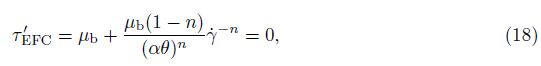
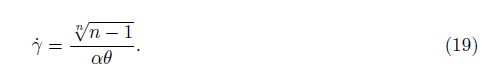
Considering that the basic viscosity μb is usually a small value, it is not a big range if n is not very close to 1. In contrast, if the material is not yielded, its effective viscosity can be very large. This division of yield and un-yield states is illustrated in Fig. 1.
In the yield like flow period (see Fig. 5(b) and Fig. 5(c)), we use short vertical lines to mark the yield surface determined through the yield viscosity criterion above. As we can see in these figures, this criterion fits the velocity profiles quite well. However, in the Newtonian like flow period (see Fig. 5(a)), because of the high initial effective viscosity, it can be considered that all the fluids are in the un-yield state. That is similar to the bi-viscosity model, in which the high effective viscosity state is considered as the un-yield state.
Because the viscosity criterion is equivalent to a microstructure criterion, the distribution of the structure parameter λ might give us a direct impression. We plot this distribution in Fig. 6, in which λc is the critical structure parameter given by Eq. (20). This figure confirms that our criterion divides the flow field into a high effective viscosity region and a low effective viscosity region quite well, except the fifth period of the flow. However, as we can see in Fig. 5, during the fifth period, the velocities of all the fluid layers tend to the wall velocity. Therefore, we can hardly say that the flow shows yield like features. Therefore, the inaccuracy of the yield surface position in the fifth period seems reasonable.

|
| Fig. 6 Distribution of structure parameter λ at different time in case that We/Re = 2 × 10⁻⁴, ReRj = 100, and λ0 = 100 |
Furthermore, we plot the shear stress on the yield surface in Fig. 7. The x-axis is time. This figure shows that there is not a fixed shear stress on the yield surface, which confirms the assertion that the stress criterion and the viscosity criterion are not equivalent to each other in this problem. In other words, a fixed yield stress does not exist, and the yield like flow case in this study is different from the traditional yield idea.

|
| Fig. 7 Shear stress-time curve on yield surface in case that We/Re = 2 × 10⁻⁴, ReRj = 100, and λ0 = 100 |
To get a better understanding of the velocity evolvement, we also draw the velocity-time curve in Fig. 8, in which the horizontal axis is time, and the vertical axis is the velocity. As we can see in this figure, all the fluids start with a static state and end up with the same wall velocity. In this progress, the fluids closer to the wall always move faster. However, their velocities do not grow monotonously, which is very different from that for Newtonian fluids. As said above, the drop of the velocity is due to the appearance of the yield region between this position and the wall. The velocity drop is small near the wall, because there is little yielded thixotropic, and it is also small or even disappears at the place that is far from the yield region. With the increase of the distance to the wall, the velocity drop appears later and lasts longer.

|
| Fig. 8 Velocity-time curves at different positions in case that We/Re = 2× 10⁻⁴, ReRj = 100, and λ0 = 100 |
There are three dimensionless parameters We/Re, ReRj, and λ0 that can affect this motion. Now, let us consider how they affect the evolvement of the flow one by one.
As we said in Section 2, We/Re determines how fast the flow field can evolve to adapt a new boundary condition or the changing of effective viscosity. We plot the velocity-time curves of different We/Re in Fig. 9. A small We/Re means a large inertial force. Therefore, as we can see in this figure that if We/Re becomes smaller, the start-up process of the velocity (from zero to the wall velocity U0) becomes slower. Large inertial forces also localize the shear near the wall. As a result, the velocity drop near the wall becomes earlier and greater, while the velocity drop far from the wall becomes weaker.

|
| Fig. 9 Velocity-time curves of different We/Re in which ReRj = 100 and λ0 = 100 |
We/Re also affects the position of the yield surface. As illustrated in Fig. 10, the inertial force enhances the shear in the flow field. Thus, it is helpful to the formation of the yield region. Therefore, the depth of the yield region increases with the decrease of We/Re at first. However, if We/Re becomes too small, the shear is localized again. Thus, the depth of yield region decreases with the decrease of We/Re when We/Re is very small.

|
| Fig. 10 Yield surface location-time curves of different We/Re in which ReRj = 100 and λ0 = 100 |
The effect of We/Re on the wall stress is shown in Fig. 11. The wall stress drop in this figure comes from the yield progress, and the yield stress is zero after the entire thixotropic fluid moves with the wall at the same velocity in the end. This figure shows that the yield progress decreases the wall stress greatly. The smaller We/Re is, the larger the wall stress is, while the earlier yield happens.

|
| Fig. 11 Wall stress-time curves of different We/Re in which ReRj = 100 and λ0 = 100 |
ReRj represents how strong the rejuvenation effect is. Rejuvenation effects decrease the fluid effective viscosity in the high shear region and cause the velocity drop. Therefore, as we can see from Fig. 12, the larger ReRj is, the earlier and stronger the velocity drop is. The rejuvenation effect is also related to the yield region. A larger ReRj always makes the yield region thicker and last longer, which is different from the effect of We/Re (see Fig. 13). Fig. 14 shows that ReRj has a similar effect upon the wall stress. A larger ReRj brings a larger wall stress and an earlier wall stress drop.

|
| Fig. 12 Velocity-time curves of different ReRj in which We/Re = 0.01 and λ0 = 100 |

|
| Fig. 13 Yield surface location-time curves of different ReRj in which We/Re = 0.01 and λ0 = 100 |

|
| Fig. 14 Wall stress-time curves of different ReRj in which We/Re = 0.01 and λ0 = 100 |
The formation of the yield region relies on the decrease of the structure parameters. Only after the structure parameters are small enough, the yield region appears. Therefore, a big initial structure parameter λ0 delays the formation of the yield region. As a result, the velocity drop is delayed. However, a larger λ0 enhances the velocity drop, because it makes the effective viscosity difference between the yield and un-yield regions greater (see Fig. 15). A smaller λ0 is helpful to the formation of the yield region. Figure 16 shows that the yield surface is higher when λ0 is smaller. An interesting result is shown by Fig. 17. Although a larger λ0 means a larger initial effective viscosity and brings a larger wall stress at first, the larger λ0 decreases the wall stress after yield. The reason is that if the initial structure parameter λ0 is large, the thixotropic fluid goes through a longer accelerating process before yield. Therefore, after yield, the un-yield region moves faster when λ0 is larger, which decreases the shear rate of the yield region and then decreases the wall stress after yield.

|
| Fig. 15 Velocity-time curves of different λ0 in which We/Re = 0.01 and ReRj = 100 |

|
| Fig. 16 Yield surface location-time curves of different λ0 in which We/Re = 0.01 and ReRj = 100 |

|
| Fig. 17 Wall stress-time curves of different λ0 in which We/Re = 0.01 and ReRj = 100 |
In summary, we present a study of the finite depth Stokes’ first problem for a thixotropic layer. The yield behavior of thixotropic fluid in this problem is investigated in detail. It is shown that, in contrast to the solution of Newtonian fluids, the velocity of the thixotropic layer generally does not increase with time monotonously during the start-up process. During the progress, the yield region appears near the wall, and the yield surface moves from the wall into the flow region and moves back to the wall finally. However, unlike simple yield stress fluids, the yield stress decreases with time in this problem. The classical solution of Newtonian fluids can be recovered from our results in extreme cases.
We/Re, ReRj, and λ0 directly affect this process. A small We/Re means a large inertial force. If We/Re becomes smaller, the start-up of the flow becomes slower, and the velocity drop near the wall becomes earlier and greater, while the velocity drop far from the wall becomes weaker. A small We/Re is helpful to the formation of the yield region but limits the yield region to a small depth when it is too small. At the same time, the smaller We/Re is, the larger wall stress is, while the earlier yield happens. ReRj represents how strong the rejuvenation effect is. The larger ReRj is, the earlier and stronger the velocity drop is. At the same time, a larger ReRj always makes the yield region thicker and last longer. A larger ReRj brings a larger wall stress and an earlier wall stress drop. A large initial structure parameter λ0 delays the formation of the yield region and delays but enhances the velocity drop. A larger λ0 decreases the depth of the yield region. Although a larger λ0 means a larger initial viscosity and brings a larger wall stress at first, a larger λ0 decreases the wall stress after yield.
The conclusions shown in this study are based on the Coussot model. Usually, this model is applied on the materials such as clay and mud. The Coussot model shows a lot of common features of thixotropic materials, such as aging, rejuvenation, and the finite characteristic time of the microstructures’ changing. Therefore, how the flow is like when the characteristic time of flow comes close to the characteristic time of the microstructures is actually a common issue for thixotropic materials. For models with other forms, the flow details are different. However, the discussion presented in this study might still be instructive.
| [1] | Barnes, H. A. Thixotropy-a review. Journal of Non-Newtonian Fluid Mechanics, 70, 1-33(1997) |
| [2] | Coussot, P., Nguyen, Q. D., Huynh, H. T., and Bonn, D. Avalanche behavior in yield stress fluids. Physical Review Letters, 88, 175501(2002) |
| [3] | Balmforth, N. J., Frigaard, I. A., and Ovarlez, G. Yielding to stress:recent developments in viscoplastic fluid mechanics. Annual Review of Fluid Mechanics, 46, 121-146(2014) |
| [4] | De Vicente, J. and Berli, C. Aging, rejuvenation, and thixotropy in yielding magneto-rheological fluids. Rheologica Acta, 52, 467-483(2013) |
| [5] | Mewis, J. and Wagner, N. J. Thixotropy. Advance in Colloid and Interface Science, 147, 214-227(2009) |
| [6] | Cheremisinoof, N. P. Encyclopedia of fluid mechanics. Rheology and Non-Newtonian Flows, 7, Gulf Publishing Company, Houston (1988) |
| [7] | Coussot, P. Rheophysics of pastes:a review of microscopic modeling approaches. Soft Matter, 3, 528-540(2007) |
| [8] | Moore, F. The rheology of ceramic slips and bodies. Transactions and Journal of the British Ceramic Society, 58, 470-494(1959) |
| [9] | Houska, M. Inzenyrske Aspekty Reologie Tixotropnich Kapalin, Ph. D. dissertation, Czech Techanical University (1980) |
| [10] | Worrall, W. E. and Tuliani, S. Viscosity changes during the ageing of clay-water suspensions. Transactions and Journal of the British Ceramic Society, 63, 167-185(1964) |
| [11] | Dullaert, K. and Mewis, J. A structural kinetics model for thixotropy. Journal of Non-Newtonian Fluid Mechanics, 139, 21-30(2006) |
| [12] | Huynh, H. T., Roussel, N., and Coussot, P. Aging and free surface flow of a thixotropic fluid. Physics of Fluids, 17, 033101(2005) |
| [13] | Liu, W. W. and Zhu, K. Q. A study of start-up flow of thixotropic fluids including inertia effects on an inclined plane. Physics of Fluids, 23, 013103(2011) |
| [14] | Chanson, H., Jarny, S., and Coussot, P. Dam break wave of thixotropic fluid. Journal of Hydraulic Engineering, 132, 280-292(2006) |
| [15] | Roussel, N., Le Roy, R., and Coussot, P. Thixotropy modelling at local and macroscopic scales. Journal of Non-Newtonian Fluid Mechanics, 117, 85-95(2004) |
| [16] | Coussot, P., Tocquer, L., Lanos, C., and Ovarlez, G. Macroscopic vs. local rheology of yield stress fluids. Journal of Non-Newtonian Fluid Mechanics, 158, 85-90(2009) |
| [17] | Billingham, J. and Ferguson, J. W. J. Laminar, unidirectional flow of a thixotropic fluid in a circular pipe. Journal of Non-Newtonian Fluid Mechanics, 47, 21-55(1993) |
| [18] | Corvisier, P., Nouar, C., Devienne, R., and Lebouché, M. Development of a thixotropic fluid flow in a pipe. Experiments in Fluids, 31, 579-587(2001) |
| [19] | McArdle, C. R., Pritchard, D., and Wilson, S. K. The Stokes boundary layer for a thixotropic or antithixotropic fluid. Journal of Non-Newtonian Fluid Mechanics, 185, 18-38(2012) |
| [20] | Stokes, G. G. On the effect of the internal friction of fluids on the motion of pendulums. Transaction of the Cambridge Philosophical Society, 9, 8-106(1851) |
| [21] | Liu, C. M. Complete solutions to extended Stokes' problems. Mathematical Problems in Engineering, 2008, 754262(2008) |
| [22] | Jordan, P. M., Puri, A., and Boros, G. On a new exact solution to Stokes' first problem for Maxwell fluids. International Journal of Non-Linear Mechanics, 39, 1371-1377(2004) |
| [23] | Fetecau, C. and Fetecau, C. A new exact solution for the flow of a Maxwell fluid past an infinite plate. International Journal of Non-Linear Mechanics, 38, 423-427(2003) |
| [24] | Tan, W. C. and Masuoka, T. Stokes' first problem for an Oldroyd-B fluid in a porous half space. Physics of Fluids, 17, 023101(2005) |
| [25] | Tan, W. C. and Masuoka, T. Stokes' first problem for a second grade fluid in a porous half-space with heated boundary. International Journal of Non-Linear Mechanics, 40, 515-522(2005) |
| [26] | Qi, H. T. and Xu, M. Y. Stokes' first problem for a viscoelastic fluid with the generalized OldroydB model. Acta Mechanica Sinica, 23, 463-469(2007) |
| [27] | Moller, P. C. F., Rodts, S., Michels, M. A. J., and Bonn, D. Shear banding and yield stress in soft glassy materials. Physical Review E, 77, 041507(2008) |
| [28] | Cheng, D. C. H. Yield stress:a time-dependent property and how to measure it. Rheologica Acta, 25, 542-554(1986) |
| [29] | Roussel, N., Le Roya, R., and Coussot, P. Thixotropy modelling at local and macroscopic scales. Journal of Non-Newtonian Fluid Mechanics, 117, 85-95(2004) |