 2016, Vol. 37
Shanghai University
Article Information
- N. NEKOUBIN, M. R. H. NOBARI. 2016.
- Numerical investigation of transonic flow over deformable airfoil with plunging motion
- Appl. Math. Mech. -Engl. Ed., 37(1): 75-96
- http://dx.doi.org/10.1007/s10483-016-2019-9
Article History
- Received Feb. 15, 2015;
- in final form Jul. 3, 2015


Flow over oscillating airfoil is encountered in many systems such as sail surfaces, compressors, wind turbines, micro air vehicles, and aircrafts. Therefore, many researchers have taken into account different aspects to investigate the flow over oscillating airfoils considering inviscid and viscous flows. This also includes the unsteady flow over airfoils with plunge, pitch, combined pitching, and plunging motion. Furthermore, previous studies have considered the unsteady flow from low to high Reynolds numbers and from subsonic flows to transonic flows using numerical and experimental methods. Gnesin and Rzadkowski[1] solved the Euler equations using the Godunov-Kolgan volume scheme to investigate the three-dimensional inviscid flutter. The dynamic stall was investigated in the study by Ekaterinaris and Platzer[2]. The unsteady, compressible, and viscous fluid flow over the NACA 0012 airfoil was studied by Murthy et al.[3]. They used the Roe scheme to explore the laminar separation. Lee and Gerontakos[4] used hot-film sensors to study boundary layer transition and separation over an oscillating airfoil experimentally. Furthermore, they discussed mechanisms responsible for the stall events. The two-dimensional heaving airfoil in a low Reynolds number was studied by Lewin and Haj-Hariri[5], in which the effects of oscillation frequency on the flow characteristics and power coefficient were investigated. Gopalakrishnan and Tafti[6] used a collocated finite volume multi block approach to study the incompressible viscous flow over the heaving airfoil. The effects of compressible flow on the heaving airfoil were investigated by Raveh and Dowell[7] considering self-sustained shock oscillation in a transonic flow over the NACA 0012 airfoil at reduced frequency and angle of attack.
Akbari and Price[8] studied the laminar incompressible viscous flow over an elliptic airfoil with pitching oscillation at a large angle of attack. They used the Joukowski transformation to solve the Navier-Stokes equations in the computational domain to investigate the influence of the oscillation frequency, the location of pitch axis, and the thickness ratio of ellipse. In their next study[9], they investigated the unsteady flow field over the pitching NACA 0012 airfoil using the vortex method to solve the Navier-Stokes equations. They concluded that the reduced frequency has a significant effect on the flow field and force coefficient of the airfoil. The influence of the pitch angle on the vertex structure and aerodynamic forces was explored in the study of Sarkar and Venkatraman[10], where they studied the dynamic stall in a wide range of the reduced frequencies. In their next study[11], they discussed the thrust generated by the pitching airfoil at high frequencies of oscillation and investigated the effects of various parameters such as the amplitude of oscillation and the location of pitching on thrust generation. Fluid flow with low Reynolds numbers over the pitching airfoil was studied by Amiralaei et al.[12]. Their study indicated the effects of aerodynamic parameters on the maximum lift coefficient and hysteresis loops of lift and drag coefficients. Also, fluid flow with high Reynolds numbers over a symmetric rotor blade with pitching oscillation was investigated by Sarkar and Bijl[13]. They studied the effects of initial conditions and structural nonlinearity. Transonic flow over the pitching airfoil was studied experimentally by Hillenherms et al.[14].
Guglielmini and Blondeaux[15] investigated the flow over a foil with a combined pitching and plunging motion, where they solved the vorticity equation for a wide range of parameters. The study by Xiao and Liao[16] investigated the effects of angle of attack profile on pitching/plunging motion. They achieved a modified cosine profile for the angle of attack. Furthermore, the particle image velocimetry (PIV) was used by Prangemeier et al.[17] to study the flow over an airfoil with plunge and quick-pitch motion. They modified the pitching/plunging oscillation using various quick-pitch motion. Ashraf et al.[18] numerically studied the effects of airfoil thickness and camber on the combined pitching and plunging airfoil considering laminar and turbulent flow regimes. Moreover, the transonic flow over the thin airfoil with pitching and plunging motion was studied by Guruswamy and Yang[19], and the transonic flow over heave/pitching flutter was experimentally investigated by Dietz et al.[20]. In addition, the Navier-Stokes equations for the transonic flow over the NACA 0012 airfoil with pitch and flap motion were solved by Iovnovich and Raveh[21]. They discussed that the aerodynamic coefficients can be regulated by planned structural motion.
The incompressible viscous flow around a flapping airfoil with active chordwise flexibility was investigated by Tay and Lim[22], where they studied the effects of flexing on three airfoil configurations and showed that flexibility does not necessarily improve the airfoil performance. Flow with low Reynolds numbers over a pitching/plunging airfoil with nonlinear deformation was studied by Jaworski and Gordnier[23]. They explored the effects of the Reynolds number variation on the vortex dynamics and aerodynamic coefficients and discussed the differences between a rigid airfoil and an airfoil with low to moderate oscillation amplitudes. Unger et al.[24] investigated the laminar-turbulent transition of incompressible fluid flow over a flapping flexible airfoil, where the effects of trailing edge deformation on the lift coefficient and the location of transition were investigated. They compared the numerical results obtained for the jig-shape of airfoil with the corresponding results obtained by the PIV measurements. The turbulent incompressible flow over an airfoil with a vertical displacement, rotation, and deformed position for aileron was studied by Svacek[25]. In this study, a reliable and robust numerical model for the simulation of fluid-structure interaction problems was presented using the finite element method and the k-ω turbulence model.
The incompressible flow over the pitching/plunging airfoil has been completely investigated in the above studies. However, the effects of airfoil deformation in the compressible fluid flow particularly at the transonic regime remain mostly unknown. Here, the unsteady transonic inviscid compressible flow over the two-dimensional deformable NACA 0012 airfoil with plunging motion is investigated numerically to explore various aspects of flow patterns. Our study covers a wide range of various parameters involved in the unsteady transonic flow. To do so, the Roe scheme in a generalized coordinates system is developed to solve the governing arbitrary Lagrangian-Eulerian equations. The effects of different governing parameters such as the phase angle, the deformation amplitude, the initial angle of attack, the flapping frequency, and the Mach number on the unsteady flow field and aerodynamic coefficients are studied in detail.
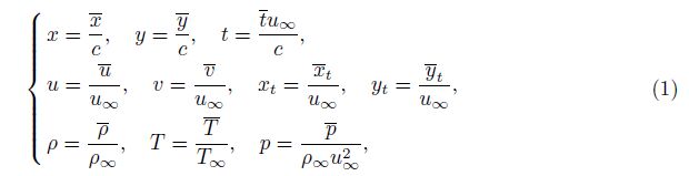
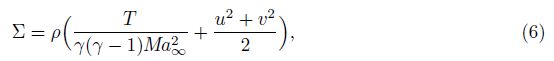
2 Governing equationsTaking into account the unsteady inviscid compressible flow over a deformable airfoil with plunging motion, the two-dimensional Euler equations in the generalized coordinates (ξ, η, t) are used. To write the equations in the non-dimensional form, the following non-dimensional parameters are used:
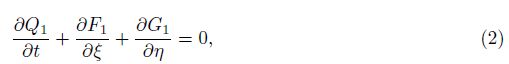
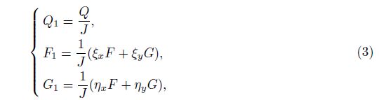
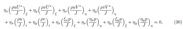
Therefore, the non-dimensional Euler equations in the conservative form can be written in the generalized coordinates as

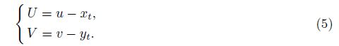
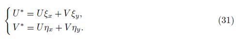
The contravariant velocities, U and V , are defined as


|
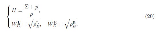
| Fig. 1 Plunging and deformable motion of airfoil (phase angle ψ = 90°, black (middle curves): down stroke; gray (upper and down curves): up stroke) |
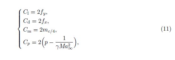
Aerodynamic characteristics consisting of the lift, drag, moment, and pressure coefficients are, respectively, as
In the present study, the Roe scheme in the generalized coordinates[27] is developed to solve the arbitrary Lagrangian-Eulerian fluid flow equations. Figure 2 shows the grid in both physical and computational domains, where the quadrilateral grids are used to maintain the non-diffuseness of the Roe scheme.

|
| Fig. 2 Grid configuration in physical domain (left) and computational domain (right) |
Here, the cell-centre method is used to store the physical quantities as shown in Fig. 3, in which the cell faces are described by dashed lines represented by E (east), W (west), N (north), and S (south). The cell faces are located at the midpoint between the nodes, and the unit vector $\hat n$ξE normal to the cell face E can be expressed as


|
| Fig. 3 Control volume in physical domain A (left) and in computational domain B (right) |
Using the first-order upwind method, we can write
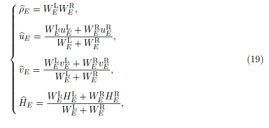
Considering Fig. 3, the Roe’s numerical flux in the generalized coordinates crossing the face E is obtained by the following equation:
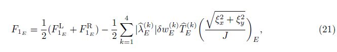
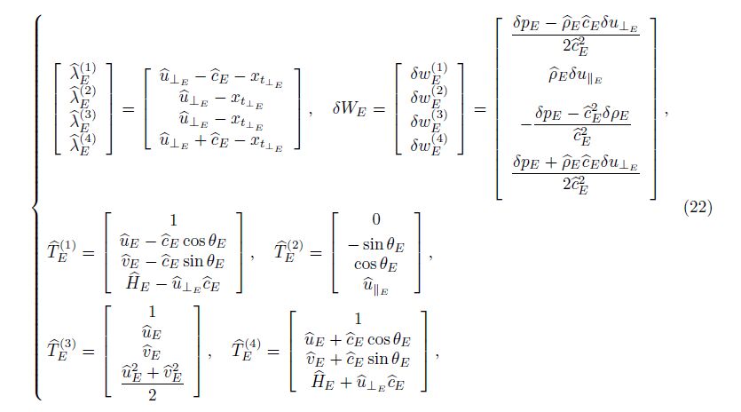
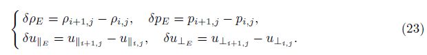
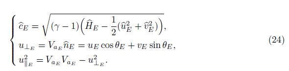
As shown in Fig. 4, u⊥E and u||E are the components of fluid velocity vectors vertical and parallel to the face E, respectively. Considering $\hat c$E as the speed of sound, we can write

|
| Fig. 4 Components of velocity vector, VaE, in xy-directions or in normal and parallel directions |
Also, xt⊥ E , the mesh velocity component vertical to the face E, is determined as

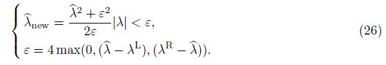
To avoid the expansion sonic waves, the following entropy correction[28] is used:
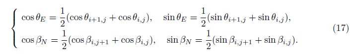
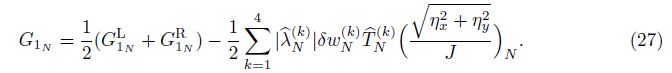
The Roe’s numerical flux in the generalized coordinates at the north face G1N is determined by the following equation:
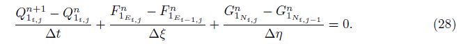
The eigenvalues, eigenvectors, and wave amplitudes at the cell face N are computed by the similar equations used for the cell face E using the β angle in the relations. By computing numerical fluxes, the Euler equation in the generalized coordinates can be discretized explicitly as follows:
In the subsonic flow, among the four eigenvalues in the two-dimensional flow, three of them are positive, and one is negative. Hence, at the inflow boundary, there are three incoming and one outgoing characteristics. As a result, three variables consisting of the velocities in the xand y-directions and the density (ρ) are specified, but the pressure (p) is extrapolated from the interior. At the outflow boundary, there is one incoming characteristic and three outgoing characteristics. Therefore, only one variable, the pressure, is specified, and the other variables are extrapolated from the interior using an explicit procedure. In the inviscid flow, the slip condition at the solid boundary is imposed. Therefore, the value of relative velocity (Vr) at the solid boundary, which is tangent to the surface as shown in Fig. 5, is assumed to be equal to its value at the point near the boundary. Consequently,
The pressure at the surface is specified by projecting the momentum equation normal to the surface, which results in the value of pressure gradient at the boundary.

|
| Fig. 5 Relative velocity vector on surface |
To determine the variables at the wall, the following iterative method[29] is used:
(i) Assume ρi, 1 = ρi, 2.
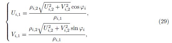
(ii) Calculate u and v using Eqs. (29) and (5).
(iii) Determine the pressure at the surface by solving Eq. (30) implicitly.
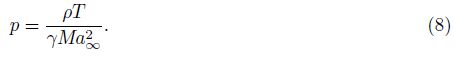
(iv) Extrapolate the temperature from the interior. (v) Use the equation of state for a perfect gas, Eq. (8), for density computing.
(vi) Check the convergence as follows:
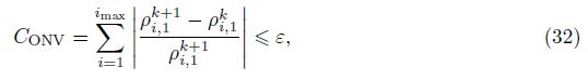
One of the important aspects of flow over a deformable airfoil with plunging motion is to handle the airfoil deformation in the computational domain. Here, we use a dynamic mesh approach to resolve the plunging and deformable motion of the airfoil. To do so, an o-type orthogonal structured mesh[29] is used, where the orthogonality of grid lines at the surface is imposed by employing a forcing function. In addition, the grid is clustered near the surface and in the vicinity of leading and trailing edges using appropriate functions. The dynamic mesh algorithm presented by Batina[30] is applied, where the spring stiffness for each edge i-j is inversely related to the length of the edge as follows:

New locations of the interior grid points are specified by solving static equilibrium equations at each time step iteratively. This is done using a predictor-corrector method, where the displacements of grid points are predicted by linear extrapolation, specified by

Then, the displacements are corrected by solving the static equilibrium equations in the xand y-directions which are given by Eq. (35). These equations can be solved by the Gauss-Seidel iteration method.
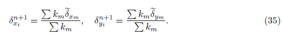
The summations in Eq. (35) are taken over 4 edges surrounding the node i. Finally, the new locations of grid points are specified by the following equations:

The grid points at the outer boundary are held fixed, while the grid points near the solid boundary up to a specified η (here 7 15ηmax) are moved by the oscillating function defined for the airfoil in Eqs. (9) and (10). Therefore, the spring method is not applied in these nodes, but it is applied for the nodes staying between 7 15 ηmax and ηmax (the outer boundary), which enables large movements to be taken into account at the higher h0 and a0 without any numerical problems. A sample of dynamic mesh used in this study is shown in Fig. 6 in eight different time intervals within a cycle of motion.

|
| Fig. 6 Dynamic mesh deformation of airfoil in eight time intervals of cycle of motion |
To avoid errors due to mesh movement, the geometric conservation law (GCL) is satisfied during the solution. Use the following expression[30]:
To show the grid independency of the numerical code developed here, three different mesh sizes at h0 = 0.1, a0 = 0.1, α0 = 2°, and ψ = π/2 are considered. The lift coefficients with respect to time for eight cycles of motion at Ma∞ = 0.755 and ω = 0.162 8 for three different meshes are presented in Fig. 7. The comparison shows good agreement of the results obtained in three different mesh sizes.

|
| Fig. 7 Time history of lift coefficient for three different mesh sizes at Ma∞ = 0.755, h0 = 0.1, a0 = 0.1, α0 = 2°, ψ = π/2, and ω = 0.162 8 |
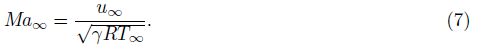
To verify the accuracy of the developed numerical method and the validation of the numerical code, the unsteady inviscid compressible flow over the NACA 0012 airfoil pitching at Ma∞ = 0.755, α0 = 0.016°, αm = 2.51°, and ω = 0.162 8 (α = α0+αmsin(ωt)) is solved. The numerical results obtained are compared with the experimental data and the numerical results of Batina[30] in Fig. 8, where the curves of the lift and moment coefficients versus the instantaneous angle of attack are shown. As it is evident from the figure, the numerical results obtained in the current study are in satisfactory agreement with the previous experimental and numerical results.

|
| Fig. 8 Comparison of lift and moment coefficients versus instantaneous angle of attack for NACA 0012 airfoil pitching at Ma∞ = 0.755, α0 = 0.016° , αm = 2.51° , and ω = 0.162 8 |
Here, the effects of different parameters such as the phase angle (ψ), the dimensionless deformation amplitude (a0), the Mach number (Ma∞), the dimensionless frequency (ω), and the initial angle of attack (α0) are investigated in the unsteady transonic compressible flow over a deformable airfoil with plunging motion in a wide range. The dimensionless plunging amplitude (h0) is fixed at 0.1, and in each case, eight cycles of motion are calculated to obtain a steady state periodic solution. Table 1 shows the effects of phase angle on the aerodynamic coefficients. Since the phase angle has slight influence on the lift and drag coefficients, it is fixed at π/2 for the remaining cases.
 |
In order to investigate the effects of deformation amplitude on the flow over the airfoil, six different values for a0 are considered from 0 to 0.25 at the intervals of 0.05. Figure 9 indicates the lift, drag, and moment coefficients versus the instantaneous angle of attack at various deformation amplitudes and flow conditions when α0 = 2°, ω = 0.162 8, and Ma∞ = 0.755. As shown in this figure, increasing the deformation amplitude causes the maximum amounts of lift, drag, and moment coefficients at the same angle of attack to increase. Consequently, the loops are enlarged for the greater a0.

|
| Fig. 9 Lift, drag, and moment coefficients versus instantaneous angle of attack for various deformation amplitudes at Ma∞ = 0.755, h0 = 0.1, α0 = 2°, ψ = π/2, and ω = 0.162 8 |
Time variations of Cl, Cd, and Cm at various deformation amplitudes are shown in Fig. 10. As it is evident from the figure, the instantaneous lift coefficients of the rigid airfoil and the deformable one vary inversely in comparison with each other, i.e., the lift coefficient for the deformable airfoil is decreased while increased for the rigid one. Furthermore, Fig. 10 indicates that the amplitudes of lift, drag, and moment coefficients are increased by the growth of the deformation amplitude. In Fig. 11, the aerodynamic coefficients of the deformable airfoil with plunging motion at different deformation amplitudes are compared with those obtained for the rigid plunging airfoil a0 = 0. It is shown that the averaged lift coefficient of the deformable airfoil is decreased by the growth of deformation amplitude. Therefore, the deformation has a negative effect on the airfoil aerodynamic performance. This effect intensifies when the deformation amplitude increases.

|
| Fig. 10 Effects of deformation amplitude on time history of lift, drag, and moment coefficients at Ma∞ = 0.755, h0 = 0.1, α0 = 2°, ψ = π/2, and ω = 0.162 8 |

|
| Fig. 11 Comparison of averaged aerodynamic coefficients of rigid airfoil and airfoil with deformation at various deformation amplitudes when Ma∞ = 0.755, h0 = 0.1, α0 = 2°, ψ = π/2, and ω = 0.162 8 |
The effects of deformation motion on the pressure distribution on the airfoil are displayed in Fig. 12, where the pressure coefficients on the upper and lower surfaces of the airfoil with the deformation amplitudes of 0, 0.1, and 0.25 at α0 = 2°, ω = 0.162 8, and Ma∞ = 0.755 are shown. As it can be seen from the figure, when the deformable airfoil with plunging motion is bent upward through the down stroke, the shock weakens on the upper surface due to the decreasing angle of attack. However, shock is relocated on the lower surface by increasing the negative angle of attack. As the airfoil moves towards its lowest position from (7+1/4)Tp to (7+1/2)Tp, the airfoil returns to its initial shape with the positive angle of attack without deformation. However, the shock remains on the lower surface and transfers from the lower surface to the upper surface with a time lag. Consequently, the lift coefficient on the large portion of down stroke is negative due to the relatively high pressure on the upper surface. As the airfoil deforms downward when bending in up stroke, shock reappears on the upper surface and strengthens by increasing the deformation. Therefore, the lift coefficient becomes positive as the shape of the airfoil reverses. Moreover, Fig. 12 shows that shocks generally strengthen as the deformation amplitude increases. Furthermore, the shock displaces remarkably over the airfoil. It is observed that the pressure difference between the lower and upper surfaces is increased as the deformation amplitude becomes larger.

|
| Fig. 12 Pressure distribution on airfoil with different deformation amplitudes within one complete motion cycle at Ma∞ = 0.755, h0 = 0.1, α0 = 2 ° , ψ = π/2, and ω = 0.162 8 |
The computed Mach contours around the deformable airfoil with plunging motion at the largest deformation amplitude, a0 = 0.25, are shown in Fig. 13 at eight different non-dimensional time within one cycle of motion. It can be seen that at t = (7+1/2)Tp, with the positive angle of attack, shock appears on the lower surface, and at t = (7+1/8)Tp, with the negative angle of attack, shock appears on the upper surface. As discussed previously, this is related to the time lag of shock displacement between upper and lower surfaces as the sign of angle of attack is changed. Moreover, at the large deformation of the airfoil, the shock appears on both lower and upper surfaces at the same time within a complete cycle of motion. This event is also shown in Fig. 12.

|
| Fig. 13 Mach contours for unsteady flow on plunging airfoil with deformation with largest deformation amplitude a0 = 0.25 at Ma∞ = 0.755, h0 = 0.1, α0 = 2 ° , ψ = π/2, and ω = 0.162 8 |
To investigate the effects of the initial angle of attack, the time histories of lift, drag, and moment coefficients are displayed in Fig. 14 at various initial angles of attack at a0 = 0.1, ω = 0.162 8, and Ma∞ = 0.755. As it can be seen from the figure, increasing the initial angle of attack causes the lift coefficient amplitude to decrease but causes the drag coefficient amplitude to increase. Moreover, the peak value of lift coefficient lags as the initial angle of attack decreases.

|
| Fig. 14 Time histories of lift, drag, and moment coefficients for various initial angles of attack at Ma∞ = 0.755, h0 = 0.1, a0 = 0.1, ψ = π/2, and ω = 0.162 8 |
In general, at the small initial angles of attack, the airfoil deformation controls the instantaneous angle of attack, and the frequency of the drag coefficient is almost twice as much as the one in the large initial angle of attack at which the instantaneous angle of attack is almost not affected by the airfoil deformation. The computed aerodynamic coefficients of the airfoil with the deformation amplitude of 0.1 at various initial angles of attack are compared in Fig. 15 to those obtained for the rigid airfoil at the same conditions. It can be seen that the averaged lift coefficient of the airfoil with deformation motion is smaller than the rigid airfoil. Furthermore, it is observed that the aerodynamic performance of the airfoil with deformation at small angles of attack is much less than the one of the rigid airfoil. However, the aerodynamic performances of the deformable airfoil and the rigid one get closer to each other as the initial angle of attack increases.

|
| Fig. 15 Averaged aerodynamic coefficients of airfoil with deformation motion at Ma∞ = 0.755, h0 = 0.1, a0 = 0.1, ψ = π/2, and ω = 0.162 8 compared to those for rigid airfoil at same flow conditions |
The effects of the flapping frequency on the aerodynamic coefficients are shown in Fig. 16 at a0 = 0.1, α0 = 2°, and Ma∞ = 0.755. As it is evident from this figure, at ω = 0.2, there is a transition point in the lift and drag coefficients trend, which appears as an inflection point in the aerodynamic performance coefficient in Fig. 17. Similarly, the computed averaged aerodynamic coefficients at various frequencies are shown in Fig. 17. It can be seen that increasing the frequency causes the averaged lift coefficient to increase and the averaged drag coefficient to decrease. Consequently, the aerodynamic performance of the airfoil improves considerably as the frequency increases. Furthermore, the slope of aerodynamic performance diagram for ω < 0.15 is slightly larger than that for ω > 0.2.

|
| Fig. 16 Time histories of lift, drag, and moment coefficients for various dimensionless flapping frequencies at Ma∞ = 0.755, h0 = 0.1, a0 = 0.1, α0 = 2 ° , and ψ = π/2 |

|
| Fig. 17 Averaged aerodynamic coefficients of airfoil with deformation motion with various dimensionless flapping frequencies at Ma∞ = 0.755, h0 = 0.1, a0 = 0.1, α0 = 2 ° , and ψ = π/2 |
Finally, the effects of the Mach number on the aerodynamic coefficients are investigated. The time histories of lift, drag, and moment coefficients at various Mach numbers for a0 = 0.1, α0 = 2°, and ω = 0.162 8 are displayed in Fig. 18. It is observed that at the Mach numbers equal or greater than 0.9, the amplitudes of lift, drag, and moment coefficients are decreased. In Fig. 19, the computed averaged aerodynamic coefficients of the deformable airfoil at various Mach numbers are compared with the corresponding values of the rigid airfoil at the same flow conditions. As it is evident from the figure, the trend in the lift coefficient of the deformable airfoil in comparison with the rigid airfoil is not monotonic. For the Mach number less than about 0.88, the lift coefficient of the rigid airfoil becomes larger than the one of the deformable airfoil. However, beyond that, the reverse effect occurs. In addition, the aerodynamic performance of the deformable airfoil degrades compared with the rigid airfoil at Ma∞ < 0.9. However, it gets closer for the two airfoils at Ma∞ ≥ 0.9.

|
| Fig. 18 Time histories of lift, drag, and moment coefficients for various Mach numbers at h0 = 0.1, a0 = 0.1, α0 = 2 ° , ψ = π/2, and ω = 0.162 8 |

|
| Fig. 19 Comparison of averaged aerodynamic coefficients for rigid airfoil and airfoil with deformation motion with various Mach numbers at h0 = 0.1, a0 = 0.1, α0 = 2 ° , ψ = π/2, and ω = 0.162 8 |
As a final point, compared the deformable airfoil and the rigid one in Fig. 15 and Fig. 19, it can be concluded that the deformable airfoil with plunging motion has more smooth and stable aerodynamic performance. Consequently, the deformable airfoil improves maneuverability.
8 Summary and conclusionsIn this article, we study the unsteady transonic inviscid compressible flow over a deformable NACA 0012 airfoil with the plunging motion. The Roe scheme in the generalized coordinates system is developed to solve the governing arbitrary Lagrangian-Eulerian fluid flow equations. A structured dynamic mesh is used to resolve the instantaneous motion of the airfoil. In a relatively wide range, the effects of parameters such as the phase angle, the deformation amplitude, the initial angle of attack, the flapping frequency, and the Mach number are investigated.
The numerical results obtained indicate that the phase angle has a negligible effect on the amplitudes and the average lift and drag coefficients. Furthermore, the deformation motion degrades the aerodynamic performance of the airfoil, and the aerodynamic performance weakens by increasing the deformation amplitude. However, the aerodynamic performance of the deformable airfoil with plunging motion stays monotone, indicating its better maneuverability compared with the rigid airfoil. Our results indicate that the aerodynamic performance of the deformable airfoil with plunging motion significantly improves by increasing the flapping frequency. In addition, at small initial angles of attack, the aerodynamic coefficient of the airfoil is remarkably affected by the airfoil deformation due to its dominant effect on the instantaneous angles of attack. However, at large initial angles of attack, the airfoil deformation has a very small effect on the instantaneous angles of attack.
| [1] | Gnesin, V. and Rzadkowski, R. A Coupled fluid-structure analysis for 3-D inviscid flutter of IV standard configuration. Journal of Sound and Vibration, 251(2), 315-327(2002) |
| [2] | Ekaterinaris, J. A. and Platzer, M. F. Computational prediction of airfoil dynamic stall. Progress in Aerospace Science, 33, 759-846(1997) |
| [3] | Murthy, P. S., Holla, V. S., and Kamath, H. Unsteady Navier-Stokes solutions for a NACA 0012 airfoil. Computer Methods in Applied Mechanics and Engineering, 186, 85-99(2000) |
| [4] | Lee, T. and Gerontakos, P. Investigation of flow over an oscillating airfoil. Journal of Fluid Mechanics, 512, 313-341(2004) |
| [5] | Lewin, G. C. and Haj-Hariri, H. Modelling thrust generation of a two-dimensional heaving airfoil in a viscous flow. Journal of Fluid Mechanins, 492, 339-362(2003) |
| [6] | Gopalakrishnan, P. and Tafti, D. K. A parallel boundary fitted dynamic mesh solver for applications to flapping flight. Computers and Fluids, 38(8), 1592-1607(2009) |
| [7] | Raveh, D. E. and Dowell, E. H. Frequency lock-in phenomenon for oscillating airfoils in buffeting flows. Journal of Fluids and Structures, 27, 89-104(2011) |
| [8] | Akbari, M. H. and Price, S. J. Simulation of the flow over elliptic airfoils oscillating at large angles of attack. Journal of Fluids and Structures, 14, 757-777(2000) |
| [9] | Akbari, M. H. and Price, S. J. Simulation of dynamic stall for a NACA 0012 airfoil using a vortex method. Journal of Fluids and Structures, 17, 855-874(2003) |
| [10] | Sarkar, S. and Venkatraman, K. Influence of pitching angle of incidence on the dynamic stall behavior of a symmetric airfoil. European Journal of Mechanics B/Fluids, 27, 219-238(2008) |
| [11] | Sarkar, S. and Venkatraman, K. Numerical simulation of thrust generating flow past a pitching airfoil. Computers and Fluids, 35, 16-42(2006) |
| [12] | Amiralaei, M. R., Alighanbari, H., and Hashemi, S. M. An investigation into the effects of unsteady parameters on the aerodynamics of a low Reynolds number pitching airfoil. Journal of Fluids and Structures, 26, 979-993(2010) |
| [13] | Sarkar, S. and Bijl, H. Nonlinear aeroelastic behavior of an oscillating airfoil during stall-induced vibration. Journal of Fluids and Structures, 24, 757-777(2008) |
| [14] | Hillenherms, C., Schröder, W., and Limberg, W. Experimental investigation of a pitching airfoil in transonic flow. Aerospace Science and Technology, 8, 583-590(2004) |
| [15] | Guglielmini, L. and Blondeaux, P. Propulsive efficiency of oscillating foils. European Journal of Mechanics B/Fluids, 23, 255-278(2004) |
| [16] | Xiao, Q. and Liao, W. Numerical investigation of angle of attack profile on propulsion performance of an oscillating foil. Computers and Fluids, 39, 1366-1380(2010) |
| [17] | Prangemeier, T., Rival, D., and Tropea, C. The manipulation of trailing-edge vortices for an airfoil in plunging motion. Journal of Fluids and Structures, 26, 193-204(2010) |
| [18] | Ashraf, M. A., Young, J., and Lai, J. C. S. Reynolds number, thickness and camber effects on flapping airfoil propulsion. Journal of Fluids and Structures, 27, 145-160(2011) |
| [19] | Guruswamy, P. and Yang, T. Y. Aeroelastic time response analysis of thin airfoils by transonic code LTRAN2. Computers and Fluids, 9, 409-425(1981) |
| [20] | Dietz, G., Schewe, G., and Mai, H. Experiments on heave/pitch limit-cycle oscillations of a supercritical airfoil close to the transonic dip. Journal of Fluids and Structures, 19, 1-16(2004) |
| [21] | Iovnovich, M. and Raveh, D. E. Transonic unsteady aerodynamics in the vicinity of shock-buffet instability. Journal of Fluids and Structures, 29, 131-142(2012) |
| [22] | Tay, W. B. and Lim, K. B. Numerical analysis of active chordwise flexibility on the performance of non-symmetrical flapping airfoils. Journal of Fluids and Structures, 26, 74-91(2010) |
| [23] | Jaworski, J. W. and Gordnier, R. E. High-order simulations of low Reynolds number membrane airfoils under prescribed motion. Journal of Fluids and Structures, 31, 49-66(2012) |
| [24] | Unger, R., Haupt, M. C., Horst, P., and Radespiel, R. Fluid-structure analysis of a flexible flapping airfoil at low Reynolds number flow. Journal of Fluids and Structures, 28, 72-88(2011) |
| [25] | Svacek, P. Numerical modelling of aeroelastic behaviour of an airfoil in viscous incompressible flow. Applied Mathematics and Computation, 217, 5078-5086(2011) |
| [26] | Shyy, W., Klevebring, F., Nilsson, M., Sloan, J., Carroll, B., and Fuentes, C. Rigid and flexible low Reynolds number airfoils. Journal of Aircraft, 36, 523-529(1999) |
| [27] | Kermani, M. J. and Plett, E. G. Roe scheme in generalized coordinates, part Ⅰ:formulations. The 39th Aerospace Science Meeting and Exhibit, American Institute of Aeronautions and Astronautics, Reston (2001) |
| [28] | Kermani, M. J. and Plett, E. G. Roe scheme in generalized coordinates, part Ⅱ:application to inviscid and viscous flows. The 39th Aerospace Science Meeting and Exhibit, American Institute of Aeronautions and Astronautics, Reston (2001) |
| [29] | Hoffmann, K. A. and Chiang, S. T. Computational Fluid Dynamics, 4th ed., Engineering Education System, Wichita, Kansas (2000) |
| [30] | Batina, J. T. Unsteady Euler airfoil solutions using unstructured dynamic meshes. AIAA Journal, 28, 1381-1388(1990) |