1 Introduction

Turbulent mixing is effectively described at various length scales. The full details of the mixture are described by the finest. Also useful is a larger scale description,in which the details of the fine scale are missing,and only average quantities come through. Since the chaotic flow we examine here is highly complex,our interest is in reduced descriptions of the flow. Many uses do not need all details of point-wise descriptions of the chaotic flow. This is fortunate as the flow is irreproducible and unstable. Statistical averages of the flow are rather significant. These will be reproducible,stable,and computable with luck directly. Thus,average quantities are involved in the reduced descriptions of the flow. Standard derivations of averaged equations lead to undefined terms which are averages of nonlinear terms. To close the averaged system, they must be modelled. This closure problem is one of essential difficulties for the multiscale multi-phase flow. Moreover,the physics level phenomena are much richer,as the averages are dependent on the length scale of averaging. We want to perform averaging over each phase and end up with the equations of multi-phase flow. Then,the forces exerted between the two phases will be reflected on the nonlinear closure terms.

Molecular mixing and chunk mixing are compressible mixing models which meet the standards of mathematical and thermodynamic consistency. In the former,the equation of state has all occurring issues of the nonlinear closure,which must describe the thermodynamic functions of an multiple species atomic mixture and the pressures. In this case,there exist common temperatures and velocities for all species. The latter is less fine grained mixing. Such a model is derived by the complete first order multi-phase averaging of the microphysical equations,in which each species has separate thermodynamics and velocities^{[1, 2, 3, 4, 5, 6]}. Here,we are concerned with the chunk mixing model for the compressible multi-phase flow involving the effect of transport and surface tension.

The purpose of this paper is twofold. Our first main result is to identify a closure satisfying all the boundary and conservation constraints in Section 4. To define closures,we propose integral identities which are based on the exact expressions for the interfacial terms. The closure proposed here is a modification and extension of Refs. ^[1]-^[3],^[7],and ^[8]. That is,it has the assumption of spatial homogeneity within the mixing zone. It follows the same physical motivations and ideas^{[9, 10, 11]}.

Our second result is a entropy inequality condition which is enforced as an equivalent condition for the positivity of an entropy of averaging,derived in Section 4. Based on the values for the closure parameters,the condition is satisfied. The newly proposed closure ensures the phase entropy conservation for smooth flows,interpreted as an entropy inequality constraint providing positivity for the entropy of averaging.

The issues raised here are possibly much wider than the particular case we study. Averaging is a fundamental tool to deal with multiscale science,whether in material science,turbulence modelling,etc. Entropy and thermodynamical relations play a leading part in such physical situations. However,even when conservation is guaranteed in an adiabatic process,a conservative formulation rarely has entropy as one of the primitive variables. It follows directly to conserve the primitive variables for the averaged equations,as these are expressed linearly and identically by the primitive variables. However,entropy is neither a primitive variable nor a linear expression in them. Thus,issues on the averaging of entropy are of importance,and these are raised extensively throughout multiscale science.

In the problems we examine,mixing is driven by accelerational forces. Richtmyer-Meshkov (RM) mixing is defined by impulsive acceleration,as by a shock wave. The classical Rayleigh- Taylor (RT) instability and the associated mixing regime are defined by steady acceleration of a density discontinuity. For an overview,see Ref. ^[12].

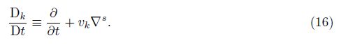
2 Governing equations

In Refs. ^[7] and ^[8] and earlier papers in this series,averaged equations have been proposed for the mixing zone interior,coupling to the buoyancy-drag equations for the motion of the mixing zone edges. A mathematical analysis of the averaged unclosed equations yields a functional form in the equations for the mixing zone interior. Closures are defined by assigning values to unknown parameters in these functional forms of the equations.

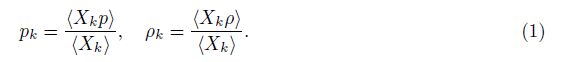
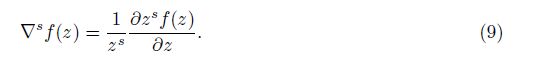
Let X_k be the phase indicator function for the material k (k = 1,2). That is,X_k(t,x) = 1 if the position x has the fluid k at the time t,zero otherwise. The microphysical Navier-Stokes equations for the compressible fluid flow are averaged by multiplication of the phase indicator function X_k. We denote the ensemble average <·>. The average <X_k>of X_k is denoted by β_k. Then,β_k(z,t) is the expected fraction of the horizontal layer at the height z that is occupied by the species k at the time t. The quantities pk and ρ_k are the phase averages of the pressure p and the density ρ,respectively,

The phase mass-weighted averages of the z-velocity vz of the fluid and the total energy E are, respectively, We also denote the internal energy e_k and the entropy S_k of the phase k as follows:

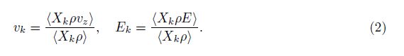
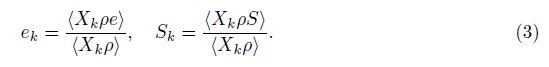
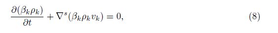
We note that a preferred direction normal to the mixing layer is chosen in the remainder of this paper. Then,the primitive equations are integrated over two other directions tangent to it. This procedure derives one-dimensional averaged equations for the multi-phase flow. Following Drew^[13] and earlier papers in the series^{[1, 2, 7]},the ensemble averaged equations are obtained,

for the velocity v_k,the volume fraction β_k,the pressure pk,the density ρ_k,and the total energy E_k of the species k. Here,g = g(t) > 0 is the gravitational force,s is the geometrical indicator, and the values 0,1,2 of s are corresponding to the planar,cylindrical,and spherical forms of the primitive equations,respectively. Summation of (5) over i yields the total mass equations, where the curvilinear divergence is To represent the source terms of (5)-(7),we use in which τ' is the viscous stress tensor,and f_k^s is the averaged geometrical source term,where f_k^s = 0 for the rectangular coordinates^[14]. hi is the specific enthalpy of the material i,ji denotes the diffusion flux^[15],and κ denotes the conductivity of heat. (∇ ·τ')_k,3 and v₃ are the third components of (∇ · τ')_k and v,respectively. Therefore,the source terms M_k,D_ki,and ε_k represent the effects of viscosity,mass diffusion,and heat conduction,respectively,so do the geometrical source terms. The models for the closure in the mixing zone interior have negligible effects of these terms. Henceforth,the terms can set to be zero to simplify the discussion. The Reynolds stress relating to the combined phases is large,and the mode equations include the effect of this term,while turbulence within a single phase is typically much smaller,and the inphase Reynolds stress is neglected on this basis. Stated alternatively,the differences of velocities between the light and heavy fluids are large,and the associated Reynolds stress exists already in the equations. The velocity fluctuation within a heavy or light fluid spike or bubble is small and can be neglected in the averaged equations. For instance,the fact is used that the velocity fluctuations of the light fluid about the mean velocity of the light fluid are small.

The interface terms are defined as

where n₃ is the unit normal vector in the preferred direction. These quantities represent averages of microscopic quantities,and these definitions are important and basic to all that follows. They are mathematically exact consequences of the averages of the primitive equations. The quantities of the right-hand side of (13) are specified to be approximated in a definition of closure to close the averaged equations (4)-(7).

We note that ∇X_k is the unit normal to ∂X_k multiplied by a delta function concentrated on the boundary ∂X_k. The definitions have the based assumption of interfacial fluxes weighted by this vector measure,which are proportional to fluxes through the direction of z only. Also for an interface quantity,for example p^∗,which may be not continuous through the interface due to surface tension,evaluation from the interior X_k side of the boundary ∂X_k is indicated by p_k^∗.

These equations are different from conventional equations for the multiphase flow in the closure forms,especially for the pressure. In the inviscid case,distinct phase pressures are assumed, and the totally hyperbolic property is shown involving the absence of complex eigenvalues for time propagation.

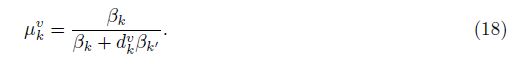
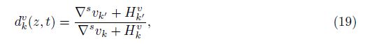
3 Closures for interfacial quantities

In Refs. ^[7] and ^[8],the convex sum formula for the interfacial quantities v^∗ and p^∗ and the fractional linear form for the mixing coefficients could be found. In addition,a natural assumption on the constitutive laws was examined to close the fractional linear form. The results are summarized in Sections 3.1 and 3.2.

We introduce the boundary conditions of the mixing zone,which should be satisfied by q^∗, q = v, p,pv closures. The height at which β₂ (β₁) vanishes is labelled the upper (lower) edge of the mixing zone,and it corresponds to the tip of the frontier portion of heavy (light) fluid in the microphysical flow. Therefore,the average q^∗ of the fluid quantity q must equal q₂ (q₁) at the upper (lower) mixing zone edge z=Z₂(t) (z=Z₁(t)). Consistency with the microscopic equations leads to the boundary conditions of the mixing zone,

For later use,we introduce the notation

for any quantity q and the notation of the convective derivative of the phase k

3.1 Closure for v^∗

The compressible v^∗ and its incompressible limit have been derived exactly from (4) and (6) independently of any closure assumption^[7]. The result is revisited as follows.

Theorem 1 The interface quantity v^∗ is in the form of the exact formula

where the mixing coefficients satisfy the fractional linear form The constitutive factor d_k^v is also expressed in the exact form where k' denotes the fluid complementary to the fluid k,i.e.,k' = 3− k,and The constitutive factor d_k^v(z,t) in (19) represents a ratio of logarithmic extent of volume creation for the two phases.

The assumption of spatial homogeneity implies a closure condition

The identity (21) means that the relative ratio of the two-fluid species volume creation does not depend on the location of space in the mixing zone. The closure (21) is thus distinct from and physically and logically independent of (19). Specifically,of course,these two formulae are distinct,but we emphasize that (21) is a closure and is not a consequence of the averaged equations,while (19) is not a closure and is a consequence of the averaged (unclosed) equations. Given the positions Z_k(t) or velocities V_k(t) = $\dot Z$_k of the mixing zone edges,the identity (21) is a zero parameter model for the constitutive factor d_k^v(t). The ratio (21) satisfies the relation d₁^v(t)d₂^v (t) = 1 which is equivalent to μ₁^v+ μ₂^v= 1. Furthermore,d_k^v(t)≥0 if and only if μv_k isnonnegative finite for 0 ≤ β_k ≤ 1.

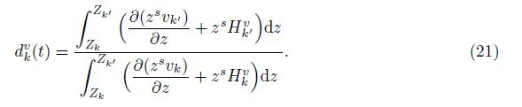
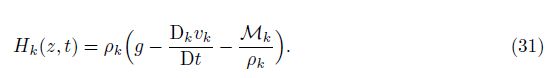
The volume creation arises primarily from the entrainment of previously unmixed pure phase fluid into the mixing zone. It affects the V_k terms in (21). Also,this effect gives rise from the relative compression of the two fluids which is a result of the logarithmic terms of substantive derivatives in (21).

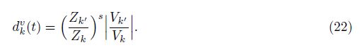
We assume that the mixing zone is expanding,i.e.,(−1)^kV_k = (−1)k $\dot Z$^k ≥0. The growing mixing zone induces the pure phase fluid to the mixture and thus yields the volume creation of the mixed fluid for both phases. In the non-diffusive RT incompressible case,the closed form solution^[10] implies the identity

In the planar case of s = 0,(22) is derived as a function of the Atwood number A = (ρ2 − ρ1)/(ρ2 + ρ1) and can be determined exactly on the basis of a theory^{[2, 16]},validated against experiments.

3.2 Closure for p^∗

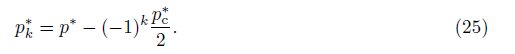
In the non-zero surface tension case,the pressure is not continuous across the interface ∂X_k, and p_k is the pressure value defined by continuity from the X_k interior. These limiting pressures at the microphysical level,i.e.,before ensemble averaging,are related by the equation

where K is the mean curvature,and σ is the surface tension. It is convenient to define so that In view of (23), p_c^∗ is the capillary pressure which is the surface tension σ times the average of the surface mean curvature. We then define the pressures

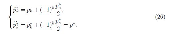
The boundary condition (14) for p^∗ at the mixing zone edge Z_k can be generalized as

which reduces to (14) in the case of zero surface tension.

The result^[7] is summarized in the following theorem.

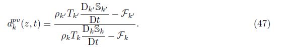
Theorem 2 The interface pressure p^∗ is expressed exactly in the form of

where the mixing coefficients μ_k^p satisfy The constitutive laws d_k^p are obtained in the exact form of where

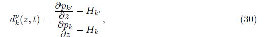
The coefficient d_k^p(z,t) indicates a ratio of the forces accelerating the two fluids,each considered in the accelerated frame and defined by their respective velocities. The pressures of two fluids become equilibrated as mixing occurs in the two fluids. At earlier time,the equilibrium is partial. In contrast,at later time,equilibrium appears in a central portion of the mixing zone, i.e., Δ$\tilde{p}$ ≈ 0. Specifically,it is shown^{[7, 8]} that the exact unclosed p^∗ in (28) has a singularity at the position z = z^∗(t) of β₁^∗ = 1/(1 − d₂^p(z,t)),where it satisfies Δ$\tilde{p}$ = 0. In addition,d_k^p(z,t) <0 when Δ$\tilde{p}$ = 0.

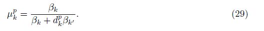
Based on the assumption of spatial homogeneity within the mixing zone,the closure is obtained by

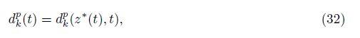
which satisfies the relation d₁^p(t)d₂^p(t) = 1 which is equivalent to μ₁^p + μ₂^p = 1. When Δ$\tilde{p}$ = 0 occurs at multiple positions,especially at later time of mixing,a zero z^∗ can be chosen as a position which appears first in the mixing zone. The closure of p^∗ with (32) is shown to be insensitive to the z^∗ choice in our data analysis.

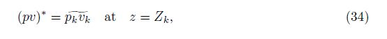
4 (pv)^∗ closure and entropy inequality

In this section,we propose a closure for the interface quantity (pv)^∗ and find an inequality constraint for the positivity of an entropy of averaging. The first step in the closure derivation is to derive an exact identity for (pv)^∗. This follows from (7) and (6) independent of (pv)^∗ closure assumptions. The result is extended here to allow for effects of multiple species mass diffusion and surface tension. Since the work associated with limiting pressures is discontinuous across the interface in the case of non-zero surface tension,from (23),we have the definition

The boundary condition (14) for (pv)^∗ at the mixing zone edge Z_k can be reformulated as where In the zero surface tension case,the condition (34) reduces to (14).

We derive a mathematically exact expression for (pv)^∗ using an entropy formulation. From (5) and (6),we obtain the kinetic energy equation

Subtracting (36) from (7),we have the internal energy equation where

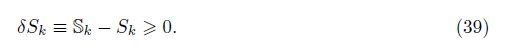
We now define S_k = S_k(E_k,ρ_k) to be the entropy defined by the averaged variables E_k and ρ_k using the equation of state,and we define S_k to be the direct ensemble average of the microphysically defined phase entropy. The process of averaging (forming the ensemble average) is not adiabatic,so that S_k ≠ S_k in general,but we expect the averaging to satisfy an entropy inequality,leading to

The averaging of in-phase fluctuations results in this difference which is identified as an entropy of averaging within a single phase. Specifically,since the averaging of the E_k and ρ_k variables is a non-isentropic process,it increases the entropy of the multi-phase flow system. For an adiabatic process,

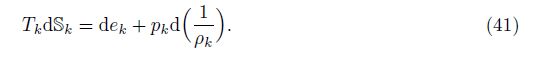
We assume that the thermodynamic relation is satisfied for the averaged quantities,

From (37) and (41),we derive the entropy equation which can be rewritten as where we define Solving (43) for (pv)^∗ yields the following theorem.

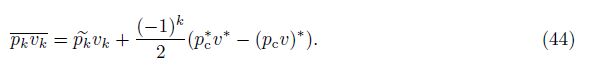
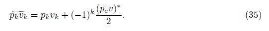
Theorem 3 The interface term (pv)^∗ is expressed exactly as

where the mixing coefficients μ_k ^pvsatisfy The constitutive coefficient d_k^pv can be obtained in the exact form Proof We sum (43) over k = 1,2 and obtain the equation for $\frac{\partial {{\beta }_{1}}}{{{\partial }_{z}}}$ Substituting (48) into (43),the exact formula (45) is obtained.

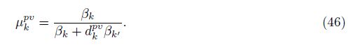
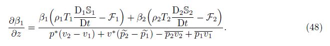
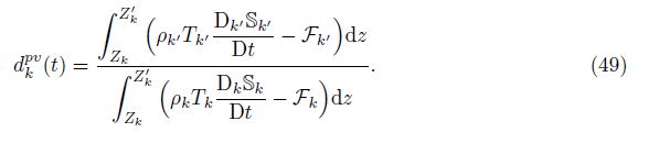
Performing the same calculations starting from the total energy closure (7) and the internal energy equation (37),we can obtain two other exact forms for (pv)^∗ and d_k^pv(z,t),respectively.These exact forms have no approximations,and they are mathematically equivalent because they are derived from the equivalent equations (43),(7),and (37). Similarly,the identities for $\frac{\partial {{\beta }_{1}}}{{{\partial }_{z}}}$ derived from (43),(7),and (37) are distinct but equivalent. As a closure condition for the quantities,we assume absence of internal length scales within the mixing zone. This assumption on one of these three equivalent identities implies three possible distinct closures for the constitutive coefficient d_k^pv . The choice selected here is the entropy form of the exact relation. This represents the ratio of the rate of heat due to the within phase averaging and suggests the closure relation

We immediately see from (49) that d₁^pv (t)d₂^pv (t) = 1 which is equivalent to the relation μ₁^pv +μ₂^pv = 1. Furthermore,d_k^pv (t) ≥ 0 is a necessary and sufficient condition for the nonnegative finite mixing coefficients μpv_k for 0 ≤ β_k ≤ 1. If $\tilde{p}$₁ ≈ $\tilde{p}$₂ ≈ p^∗,then (pv)^∗ ≈ p^∗v^∗ is independent of d_k^pv .

The process of ensemble averaging increases the entropy of the system,a process we call the positive entropy of averaging property. When the source term F_k = 0,we expect that the entropy of averaging is positive,which leads to the following theorem.

Theorem 4 Assume the closures (17),(28),and (45) for v^∗, p^∗,and (pv)^∗. Assume the source term F_k = 0. Then,the equivalent constraint for the entropy of averaging inequality $\frac{{{D}_{1}}\delta {{S}_{k}}}{Dt}$ ≥0 for the k = 1 and k = 2 fluids is

Proof From (43),(6),and (40),we obtain the equation

for the difference δS_k. Summing (51) over k = 1,2 shows that is the necessary condition for the k = 1 and k = 2 flows to have nonnegative entropy of averaging source terms. We note that there is no contribution of the (pv)^∗ closure to (52). With (17) and (28),(52) easily reduces to (50). Now,we assume (50). We prove that the closures satisfy the inequality which is equivalent to having nonnegative source terms in (51). Define Then,(53) is rewritten in the form of Notice that C1 ≤ C2 directly follows from (50). From the assumed validity of (50),and the linear combination laws (17),(28),and (45) for v^∗, p^∗,and (pv)^∗,we obtain Similarly, 5 Conclusions

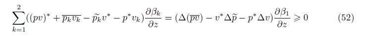
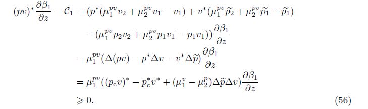
The p^∗ and v^∗ closures^[7] repeated in Section 3 and the newly proposed (pv)^∗ closure in (45) and (49) satisfy all the requirements for conservation and boundaries. The boundary condition at the mixing zone edge is given in (14). Since an averaging process is not adiabatic, conservation of entropy should not be satisfied,but the enforced entropy inequality constraint (50) imposes the nonnegative entropy of averaging. Conservation of total energy is ensured by (7). From (5) and (6),conservation of species mass and total momentum for rectangular geometry is guaranteed in the absence of diffusion and viscosity.