1 Introduction

Saturated soil can be modeled as a two-phase medium (a poroelastic medium). Researchers and engineers have used the poroelastodynamics theory to study seismicity,earthquake engineering,geophysics,and acoustics for several decades. The development of the theory and its applications can be found in the standard literature^{[1, 2, 3, 4, 5, 6, 7, 8, 9, 10]}.

The poroelastodynamics theory was pioneered by Biot^{[1, 2]}. The theory assumes a linear elastic porous solid undergoing small deformation with a fluid flow governed by Darcy’s law. Biot predicted the propagation of two dilatational waves and one distortional wave in this two-phase porous medium. The prediction has been observed in the laboratory by Plona^[11],Ding^[12],and Plona and Johnson^[13].

Most of the studies of poroelastodynamics were done in the frequency domain,because the results are easier to be obtained,and the time domain solution can be constructed using the Fourier transform. Previous works include Refs. ^[14]-^[23].

The benefits of the computational methods applied to poroelastodynamics have been reviewed by Schanz^[24]. The boundary element method (BEM) has the advantage of reducing the number of dimensions in the computation,and using Green’s functions as the weighing function of the integral equations produces more accurate results. The superposition of Green’s functions also satisfies the radiation condition at the far field. Hence,the BEM provides a useful and effective tool for computational soil dynamics. For a specified group of problems,the BEM is also amenable for treatment of computational technology such as the object-oriented programming^[25].

Cheng et al.^[4] presented Green’s functions of poroelastodynamics utilizing an analogy between the dynamic thermoelasticity and the dynamic poroelasticity in the frequency domain. The solution was presented as the u-p formulation,as the corresponding quantity to the temperature was the pore pressure. In this work,we present a new methodology for deriving Green’s functions,which has the advantage of decoupling the fast and slow dilatational waves. The methodology is the same as that presented by Ding et al.^[26]. However,a special term “decoupling coefficient” (for the fast and slow dilatational waves) is proposed and expressed in this paper. Based on the formulation,we then carry out the numerical implementation and plot these curves based on a set of parameters. The correctness of the solution is demonstrated by numerically comparing the current solution with Cheng’s previous solution. The separation of the two dilatational waves in the present methodology allows them to be more accurately evaluated than they are combined. This accuracy is particularly useful for the slow wave,whose magnitude decay is much quicker than that of the fast wave. This can be advantageous for numerical implementation in methods like the BEM and in other applications.

2 Governing equations and Green’s functions of dynamic poroelasticity

Biot’s governing equations for the dynamic poroelasticity are as follows^{[1, 2]}:

The constitutive equations are

The equilibrium equation is

The generalized Darcy’s law of the fluid phase is

where

The continuity equation of the fluid phase is

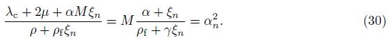
In the above,λ and μ are Lam$\overset{'}{\mathop{e}}\,$ constants,α is Biot’s effective stress coefficient,and M is Biot’s modulus,which is the inverse of a storage coefficient,u and w are the displacement of the solid phase and the average displacement vector of the fluid phase relative to the solid phase,respectively ($\ddot u$ = d²u/dt²,$\ddot w$ = d²w/dt²),ρ and ρ_f are the total mass density (combined solid and fluid phases) and the fluid mass density,respectively (ρ = (1−β₀)_ρs+β_0ρf,where ρ_s is the mass density of the solid phase). ρ_a is the apparent mass density. β₀ is the porosity. λ_c,μ,α,and M are four independent poroelastic constants. We also note that e_ij = (u_i,j + u_j,i)/2 is the strain tensor of the solid phase,and e = e_ii is the volumetric strain of the solid phase. The relative volumetric strain of the fluid phase is w_i,i. u_i and w_i are components of u and w in the ith direction,respectively. If a medium is always in a saturated situation in the dynamic process,we have $\dot w$ _i,i = q_i,i in Eq. (6). ζ = −w_i,i is the variation in the fluid content,and χ is a fluid source. Other terms include: σ_ij ,the total stress; p_,i,the gradient of the pore pressure in the ith direction; F_i and f_i,the body forces of the solid and fluid phases in the ith direction,respectively; κ = k/η,where k is the permeability,and η is the dynamic viscosity of the fluid; and δ_ij ,the Kronecker delta with i,j = 1,2,3. For Biot’s parameters α and M,we find the following relations:

where v is Possion’s ratio,v_u is the undrained Possion’s ratio,and B is Skempton’s pore pressure coefficient.

The above equations can be combined to give the following two coupled equations for the dynamic poroelasticity^[4]:

where λ_c = λ+α²M. In the frequency domain,dropping the body force terms for now,Eqs. (8) and (9) become where ${{\tilde{u}}_{i}}$ and ${{\tilde{w}}_{i}}$ are the Fourier transforms of u_i and w_i,respectively,and δ_ikh and δ_hlj are the permutation tensors with k,h,l = 1,2,3. We can recast Eq. (11) as That is, where i is the unit of imaginary number.

(i) Components of non-divergence field

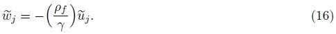
If $\tilde{u}$ and $\tilde{w}$ in Eq. (11) are the components of the non-divergence field,we can derive the following:

Substituting Eq. (16) into Eq. (10),we obtain Thus, where β represents the velocity of distortional wave,

(ii) Components of irrotational field

If $\tilde{u}$ and $\tilde{w}$ are the components of the irrotational field,we can suppose

where n = 1,2,and α₁ and α₂ are the velocities of the fast and slow dilatational waves,respectively. Substituting Eqs. (19)-(21) into Eqs. (10) and (11),we obtain

Equations (23) and (24) can be put into the forms that are more suitable for describing the wave equations as follows:

where

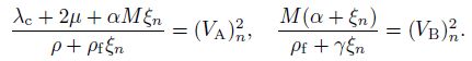
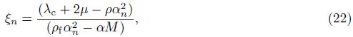
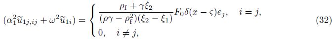
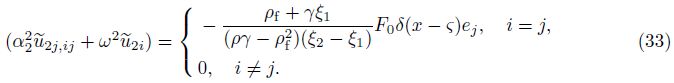
As analyzed by Biot^[1],there exist only two irrotational waves,i.e.,one fast dilatational wave and one slow dilatational wave. Therefore,we have

Then,Eqs. (25) and (26) can be written as and

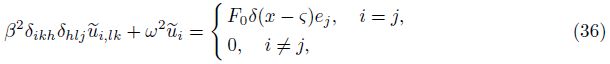
If a concentrated force${{\tilde{F}}_{j}}$ = F₀δ(x − ς)e_j (where F₀ is the magnitude of force,e_j is a unit vector in the jth direction,and δ is the Dirac delta function) is assumed to act at a point ς in a poroelastic medium,Eq. (28) can be written as

where x is the coordinate of the field point. Equations (31) and (29) are two simultaneous equations,which allow us to solve for the following equations:

Hence,we have the following familiar classical solutions:

In Eqs. (34) and (35),K_αn = ω/α_n are the wave numbers of the fast or slow dilatational wave,and r = |r| = |x − ς| is the distance between the source point and the field point.

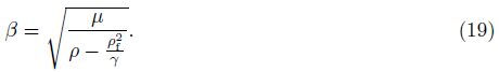
Similarly,we can obtain the solution of the distortional wave from Eq. (18)^[23],

where K_β is the wave number of the distortional wave,and K_β² = ω²/β². Then,the solution of Eqs. (10) and (11) is as follows^[23]: In Eq. (37),the 1/r terms can be cancelled out,and it can be expressed as the form of Fourier’s spectrum of Green’s function G_ij (x/ς,ω) as follows (as $\tilde{u}_{ij}^{f}$ in Cheng et al.^[4]): where

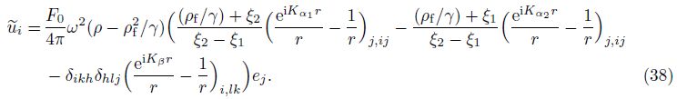
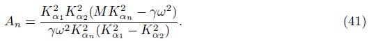
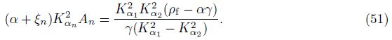
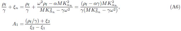
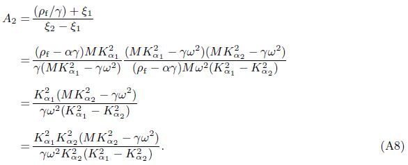
We can define A₁ and A₂ in Eq. (40) as “decoupling coefficients” for decomposition of the fast and slow dilatational waves of Eq. (12). Equation (40) is also the expression of “decoupling coefficients”. The form of G_ij(x/ς,ω) was written as $\tilde{u}_{ij}^{f}$ by Cheng et al.^[4]. Based on a deduction procedure shown in Appendix A,Eq. (40) can be recast as

3 Green’s function for fluid phase 3.1 G_4i( x/ς,ω)

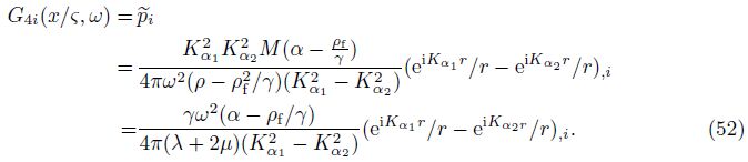
G_4i(x/ς,ω) (as $\tilde{p}_{j}^{f}$ in Cheng et al.^[4]) is defined as the pore pressure at the field point x due to a unit concentrated force acting at the source point ς in the ith direction. From Eqs. (11) and (3),we have^[25]

where T is the duration of influence from the fluid source. Since injection of the fluid source is not considered here,the last term of the right-side in Eq. (42) vanishes with χ = 0. Therefore,we have As the fluid has no shear strength,the non-divergence components of $\tilde{u}$ and $\tilde{w}$ have no effect on the fluid phase. Thus,the component of $\overset{\tilde{\ }}{\mathop{u}}\,$ in the irrotational field subjected to a unit force from Eq. (38) can be obtained as follows:

Employing Eq. (21),we obtain the component of the irrotational field $\tilde{w}$ subjected to a unit force as follows:

The corresponding divergence can be obtained as

Substituting Eqs. (46)-(49) into Eq. (43),we are ready to write a concise result,

where In Appendix A,the various expression of Eq. (51) is analyzed in detail. Thus,we have

3.2 G_i4(x/ς,ω) (as $\tilde{u}_{i}^{s}$ in Cheng et al.^[4])

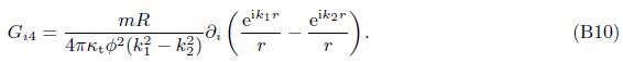
G_i4(x/ς,ω) is defined as the displacement at the field point x in the ith direction due to the injection of a unit volume of fluid into the pore at the field point ς. There is a simple expression derived from Betti’s theorem of reciprocity as follows:

In the frequency domain, Therefore,we obtain the solution readily

3.3 G₄₄(x/ς,ω) (as ${{\tilde{p}}^{s}}$ in Cheng et al.^[4])

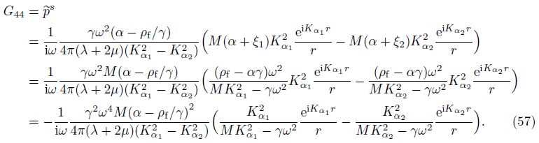
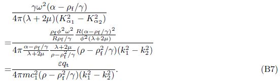
Similar to G_i4(x/ς,ω),G₄₄(x/ς,ω) is defined as the pore-fluid pressure at the field point x due to the injection of a unit volume fluid at the source point ς. Employing the definition of G_i4 and Eq. (43),we can obtain

where the subscript n = 1,2. The summation convention for the Cartesian tensors has been used in Eq.(56),ξ_nG_i4(n) = ξ₁G_i4(1) + ξ₂G_i4(2); G_i4(n)represents the corresponding part of G_i4 which belongs to the fast dilatational wave (n = 1) or the slow dilatational wave (n = 2),respectively. Substituting Eq. (55) into Eq. (56),we can obtain the result after some derivations presented in Appendix B, Equations (39),(52),(55),and (57) are identical for the corresponding Green’s functions of a poroelastic medium obtained by Cheng et al.^[4] via analogy with the dynamic thermoelasticity. The correspondences between the current solution and that in Ref. ^[4] are shown in detail in Table 1 and Appendix B. In Table 1,we define the notations by

4 Numerical implementation for comparison

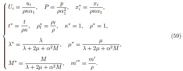
As the approaches and the various notations are different in the current paper and Ref. ^[4],it is important to compare the numerical results of the two solutions. For convenience,the dimensionless displacement,the pore pressure,and the relevant physical parameters are defined as follows^{[27, 28]}:

4.1 Results of numerical implementation by original dimensional parameters of Table 2

The original dimensional parameters and the corresponding values are shown in Table 2. The dimensionless homologous parameters substituted into formulas for computation are λ^* = 0.171 5,μ^* = 0.300 7,M^* = 0.374 2,α = 0.779,κ^* = 1,ρ^* = 1,and ρ_f^* = 0.432 5^{[27, 28]}. For the source point ς^* = (0,0,0) and the field point x^* = (0.1,0.15,0.2) ,the results of numerical implementation are shown in Figs. 1-6. The dashed lines are the results in Ref. ^[4]. Good agreement between the corresponding curves can be easily assessed.

4.2 Results of numerical implementation by original dimensional parameters of Table 3

In order to further confirm the stability of the numerical implementation,we change the dimensionless parameters to λ^* = 0.128 6,μ^* = 0.274 6,M^* = 0.467 9,α = 0.83,and ${{m}^{'*}}$ = 2.256. The dimensionless parameters ρ^*,ρ_f^* ,κ^*,and the coordinates of the source point and the field point are maintained. The computational results are shown in Figs. 7-12. The dashed lines are results obtained by Cheng et al.^[4]. Similarly,good agreement between the corresponding curves can be easily assessed.

5 Discussion

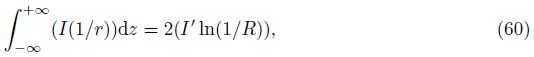
(i) The above presented results are three-dimensional. The two-dimensional (plan strain) Green’s functions can also be useful in many applications. De Hoop^[29] proposed that the two-dimensional Green’s function can be obtained by integrating of the three-dimensional Green’s function over the x₃-axis (z-axis). Manolis^[30] proved that De Hoop’s method was feasible and accurate. Ding et al.^[31] integrated the three-dimensional Green’s functions with respect to the x₃-axis in (−∞,+∞) to obtain the two-dimensional Green’s functions of solid phase. In fact,for the two-dimensional Green’s functions,we should pay attention to the following identity:

where I and r stand for a unit matrix and the distance between the source point and the field point in a space (3D) coordinate,respectively,$r=\sqrt{{{x}^{2}}+{{y}^{2}}+{{z}^{2}}}$,and ${{I}^{'}}$and R stand for a unit matrix and the distance between the source point and the field point in a plane (2D) coordinate,respectively,and $R=\sqrt{{{x}^{2}}+{{y}^{2}}}$. Employing the aforementioned identity and applying some similar processes as in Sections 2 and 3,we can readily find that the twodimensional Green’s functions of a poroelastic medium in the frequency domain obtained by Cheng et al. via analogy between the dynamic thermoelasticity and the dynamic poroelasticity are valid and concise,and successful for u-p formulation^[26] also.

(ii) Equations (38) and (39) are the solutions of Philippacopoulos’s paper^[21] also,but these are not Green’s functions of the fluid source as claimed by Philippacopoulos. The solutions in Ref. ^[4] are the complete results for the u-p formulation of solutions of Biot’s dynamic equation.

6 Conclusions

Based on Green’s functions of the displacement field for the solid and fluid phases of poroelastodynamics presented in this paper,we can make the following conclusions:

(i) The solutions of Green’s functions with the concentrated force which is provided by Cheng et al.^[4] are valid and concise. They can be effectively used in the frequency domain for the numerical implementation of dynamic poroelastic problems.

(ii) Analogy between the dynamic thermoelasticity and the dynamic poroelasticity in the frequency domain may be an important approach to solve complex problems pertaining to the corresponding poroelastic governing differential equations.

(iii) The expressions associated with the decoupling of the fast and slow dilatational waves in this paper (Eq. (40)) (decoupling coefficients) will be beneficial in the research of poroelastodynamics.

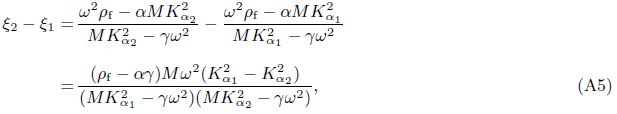
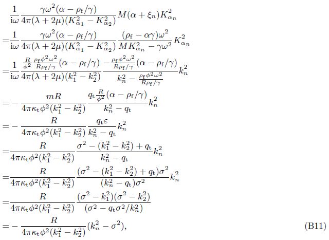
Appendix A

Employing Eqs. (25) and (26),we have

where n = 1,2. The solutions of the above quadratic equations are where Recasting Eq. (27),we can write Thus,the following equivalent relations can be satisfied: Consequently,we can readily obtain

Appendix B

The solutions of Green’s functions deduced in the current paper differ in forms from the results obtained by Cheng et al.^[4] ,but they are in fact identical.

We can define

In addition,we have Substituting the relation formula σ² = ω²/c₁² into Eqs. (A9) and (A2),respectively,and utilizing K_{α 1}²K_{α 2}² = qtσ2,we have If we express k₁ = K_α1 ,k₂ = K_α2,and τ = K_β,then Eq. (37) becomes Equation (B6) is the $\tilde{u}_{i}^{f}$ expression provided by Cheng et al.^[4]. Moreover, Therefore,Eq. (51) is For G_i4,we can obtain Therefore,Eq. (51) is For G₄₄,we have Equations (B7),(B10),and (B12) are the expressions $\tilde{p}_{j}^{f}$,$\tilde{u}_{i}^{s}$ ,and ${{\tilde{p}}^{s}}$ provided by Cheng et al.^[4] ,respectively.