1 Introduction

It is very important to simulate linear elasticity problems in science and engineering, such as numerical simulation of many-body problem of microelectronic mechanical systems, which often needs to do some elastic analysis^[1]. However, due to the complexity of problems and regions, generally, it is difficult to get the analytical solution. Therefore, the finite element method has become one of the most commonly used numerical methods to simulate linear elasticity problems^{[2, 3]} at present. In practical applications, there are many factors which cause various singular solutions to elasticity problems, such as non-smooth physical regions (the concave angle or crack), discontinuous material constants, and stress concentration. Although these singularities can be overcome by the numerical method based on the uniform refinement mesh, the physical memory and CPU time of computers can increase severely. This is because that the number of degree of freedom based on the uniform refinement mesh increases exponentially. The adaptive finite element method (AFEM) can avoid these effects by adjusting grid points according to the properties of solutions and obtain the largest calculation accuracy with the minimum amount of computation. Therefore, this method has a wide range of applications in the modern engineering calculation^{[4, 5, 6, 7, 8, 9, 10]}.

At present, the adaptive method based on the Zienkiewicz-Zhu type posteriori error estimation is widely used in engineering calculation^{[6, 7, 8, 9]}, and the corresponding theoretical analysis can be found in a great number of research works^{[4, 10, 11, 12, 13]}. To construct the posteriori error estimator^[14] and the adaptive finite element algorithm for the H1 scalar elliptic equation^[15], an AFEM has been designed in Ref. ^[16] with non-special treatment of oscillation and a minimal element refinement without interior node property for linear elasticity problems in two dimensions. The corresponding convergence analysis has been given in Ref. ^[17]. The main purpose of this paper is to present the quasi-optimal complexity by consulting the quasi-optimal complexity^[15].

In this paper, in addition to a special constant, we always adopt the mark a \lesssim b, which indicates that there is a constant C such that a ≤ C_b, and a ≈ b indicates a \lesssim b and b \lesssim a at the same time.

2 Model problem and AFEM 2.1 Model problem

Let Ω be a bounded and Lipschitz domain in R², ∂Ω = Γ_D ∪ Γ_S, and Γ_D ∪ Γ_S = ∅ Let n = (n_x, n_y)^T be a unit normal vector of ∂Ω , u :Ω → R² be a displacement vector, and f be an external force. We consider a linear elasticity problem

where Here, λ and μ are the Lamé constants, which can be composed, respectively, by the elastic modulus E and Poisson’s ratio ν, i.e.,

Introduce the following finite element spaces:

The variational formulation of problems (1)-(3) is to find u ∈ (H_ΓD¹(Ω))² such that

where

Assume that Ω is covered by a regular mesh of triangle T . We introduce the following finite element space of order p:

where P_p(τ) denotes the space of homogeneous polynomials of order based on τ.

Using the finite element space of order p, we introduce the following discrete variational problem of (4): find u_T^(p) ∈ V^(p)(T ) such that

Notice that V^(p)(T ) is the proper subspace (H_ΓD¹(Ω))². We know that the discrete variational problem (5) is well-posed. Because the bilinear form a(·, ·) is positive and coercive, we can induce an inner product 〈u, v〉 = a(·, ·) based on (H_ΓD¹(Ω))², and the corresponding energy norm satisfies where these positive constants C and c depend on λ and μ.

2.2 AFEM

In this subsection, we give a brief introduction of the standard AFEM^[15]. Let T₀ be a conforming triangular grid on the bounded domain Ω, and let {T_k}_k>0 be a sequence of nested and conforming grids by a series of local refinement. The grid T_k+1 is generated from T_k by the following algorithm modules of AFEMs:

(1) SOLVE

For the given functions f, g, g_S, and a given conforming grid T_k, we assume that the algorithm module SOLVE exactly outputs the discrete solution u_k^(p) of (5) as

(2) ESTIMATE

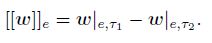
Let ε(T_k) be the set of the interior edges of grid T_k. For any edge e ∈ ε(T_k) shared by two triangle elements τ₁ and τ₂, we define the inter jumps of a vector function w across the edge e as follows:

Especilly, when e ∈ Γ_S, we define [[w]]_e = w|_e.

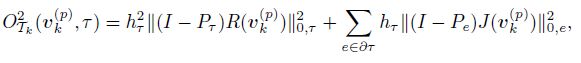
Let n_e = (n_x, n_y)^T be a unit normal vector across the edge e. For a given triangle element τ ∈ T_k and a given function v_k^(p) ∈ V_k^(p) , the posteriori error estimator based on τ is given by

where h_τ = |τ|^1/2, R(v_k^(p) )|_τ := f|_τ - Lv_k^(p) |_τ , and J(v_k^(p) )|_e := [[L^T(n_x, n_y)DL(∂_x, ∂_y)v_k^(p)]]_e.

For any element subset M_k ⊂ T_k, we define

Especially, we simply define η²(v_k^(p) , T_k) = η²T_k (v_k^(p) , T_k) when M_k = T_k.

For any given triangle grid T_k and the corresponding discrete exact u_k^(p) ∈ V _k^(p) of (5), we can obtain the posteriori error estimator η²T_k(u_k^(p) , τ) of any triangle element τ ∈ T_k by the following algorithm module:

(3) MARK

In this paper, we utilize the Dörfler marking way^[18] to mark elements which will be refined. Given a triangle grid T_k, a set of posteriori error estimators {η²T_k(u_k^(p) , τ)}∈T_k , and a Dörfler marking parameter ϑ ∈ (0, 1), we can get a marked element set M_k ⊂ T_k by the following algorithm module:

In addition, the set M_k satisfies and has a minimal cardinality.

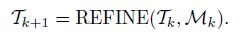
(4) REFINE

In this paper, we refine these marked triangle elements by way of newest vertex bisection. A detailed introduction about the newest vertex bisection was provided in Ref. ^[19]. In order to prove the quasi-optimal complexity, we introduce this bisection briefly. Given a simplex τ and a labeled refinement edge, we describe the following mapping:

where τ₁ and τ₂ are two new simplices, and e₁ and e₂ are the edges opposite to the newest vertexes of τ₁ and τ₂, respectively.

Given a labeled initial grid T₀ and a bisection method, we define a set as

where the instruction about the addition T₀ + B was given in Ref. ^[19].

Namely, F(T₀) contains all grids obtained from T₀ using the newest vertex bisection method. However, a grid T ∈ F(T₀) can be non-conforming. Thus, we define C(T₀) as a subset of F(T₀) containing only conforming grids.

Being the same as the assumptions in Ref. ^[19], we consider the newest vertex bisection method which satisfies the following two assumptions:

(i) For any T ∈ F(T₀), T is shape regular.

(ii) The uniformly refined grid $\bar T$_k ∈ C(T₀) is conforming for all k > 0.

We assume that a module REFINE implements an iterative or a recursive bisection (see Refs. ^[20] and ^[21]), and the initial grid T₀ satisfies the assumptions (i) and (ii). For a given number k ≥ 1, any grid T_k ∈ C(T₀, and a subset M_k ⊂ T_k, we can obtain a conforming grid T_k+1 ∈ C(T₀ by the algorithm module REFINE as

In order to obtain T_k+1, we bisect all triangle elements of the set M_k. Then, we get a new grid T ′k+1. Generally speaking, the grid T ′ _k+1 6= T_k+1, and it may include a number of hangedpoints. We have to bisect some other triangle elements of T_k \M_k and obtain the conforming grid T_k+1. However, the number of these extra refinement elements cannot be controlled by C#M_k, where C is a constant, and #M_k represents the cardinality of M_k. In fact, there is a constant C_k which can rely on the refinement times r and $\mathop {\lim }\limits_{x \to \infty } $C_k = ∞ such that

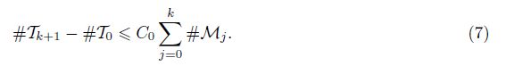
Fortunately, there is the average form about (6).

Theorem 1^{[21, 22]} Assume that the bisection satisfies the assumptions (i) and (ii). Then, there exists a constant C₀ which only relies on the shape regular mesh T₀, and

Using the above four algorithm modules, we design an AFEM, in which the refinement mesh does not need to satisfy the “internal nodes” property and does not need to mark the oscillation (AFEM algorithm^[16]).

Algorithm 1 (AFEM) For given functions f, g, and g_S, choosing a Dörfler marking parameter ϑ ∈ (0, 1) and an error control constant etol, the modules of AFEM algorithm are as follows:

(i) Give an initial conforming triangle grid T₀ and set k = 0.

(ii) u_k^(p) = SOLVE(T_k, f, g, gS).

(iii) η²T_k(u_k^(p) , τ) = ESTIMATE(T_k, u_k^(p) , f, g, g_S). If η²(u_k^(p) , T_k) < etol, then the algorithmstops.

(iv) M_k = MARK(η²(u_k^(p) , T_k), T_k, ϑ).

(v) T_k+1 = REFINE(T_k, M_k).

(vi) Set k = k + 1, and go to (ii).

The algorithm above is convergent, and it has been proved in Ref. ^[17]. In the next section, we shall testify the corresponding quasi-optimal complexity.

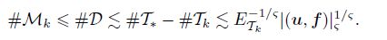
3 Quasi-optimal complexity

In this section, given an initial conforming triangle grid T₀ and a Döfler marking parameter ϑ ∈ (0, ϑ_∗), the AFEM algorithm is of the quasi-optimal complexity about degree of freedom.

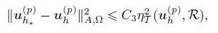
To prove the quasi-optimal complexity, we need a global upper bound for the distance between two nested solutions. Because the lower bound involves oscillation, we shall introduce its definition. For any triangle grid T_k ∈ C(T₀ and any element τ ∈ T_k, we define the oscillation v_k^(p) ∈ V _k^(p) as

where P_τ is the L²-projection onto the set of piecewise polynomials (P_p)² over τ, and also P_e is an L²-projection onto the set of piecewise polynomials dP_p over e.

Like the error estimator, for any subset of M⊆ T_k, we define the oscillation of M as

Specially, when M= T_k, we use a simplified O(v_k^(p) , T_k).

Using the definitions of the error estimator and oscillation, the property of the local L²-projection and the monotonicity of local mesh sizes, we can obtain the following lemmas easily.

Lemma 1 Let T_k ∈ C(T₀ and v_k^(p) ∈ V_k^(p) be given. We have the following results.

(i) For any τ ∈ T_k, the oscillation OT_k (v_k^(p) , τ) is dominated by the posteriori error estimator ηT_k (v_k^(p) , τ).

(ii) In view that the definitions of the posteriori error estimator and oscillation are fully localized to τ ∈ T_k, for any τ ∈ T_k+1, there hold

where T_k+1 ∈ C(T₀.

(iii) Assume that the triangle grid T_k+1 is any refinement of T_k. Then, by combining the monotonicity of local mesh sizes and properties of the local L2-projection, we deduce the monotonicity properties

where T_k+1 ∈ C(T₀.

Before discussing the global upper bound, we introduce some standard bubble functions. Let B_τ and B_e denote the element bubble functions corresponding to the element τ and the edge e, respectively. We shall use the following inequalities about the bubble function.

Lemma 2 For any τ ∈ T , e ⊂ ε_h, and v_h^(p) ∈ V_h^(p) , we have

where the above constants depend only on the shape regularity of element τ.

The following lemma presents some special properties for the bilinear a(u-u_k^(p) , v_k^(p) ) with any function v_k^(p) ∈ V_k^(p) , where u ∈ H_ΓD¹(Ω) and u_k^(p) ∈ V_k^(p) are the solutions of (4) and (5), respectively.

Lemma 3 Given a triangulation T ∈ C(T₀. Let u ∈ H_ΓD¹(Ω) be the solution of (4), and let u_k^(p) ∈ V _k^(p) be the discrete solution of (5). Then, the following results are obtained.

(i) For any τ ∈ T_k and v ∈ H¹(τ) with supp v ⊂ τ, we have

(ii) For any e ∈ ε_k and w ∈ H¹(e) with suppw ⊂ Ω_e, we have

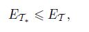
Using Lemmas 2 and 3, we can present the global lower bound for the posteriori error estimator.

Lemma 4 (Global lower bound) Given a triangle grid T_k ∈ C(T₀, let u be the solution of (4), and let u_k^(p) ∈ V _k^(p) be the discrete solution of (5). There exists a constant C₂ > 0 such that

The constant C₂ > 0 only depends on the shape regularity of T_k and the constants λ and μ.

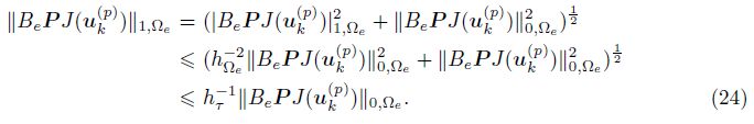
Proof For any triangle element τ ∈ T_k, we shall estimate h_τ²║R(u_k^(p) )k║_{0, τ}² and h_τ║J(u_k^(p) )║_{0, e}², respectively.

Firstly, we shall estimate h_τ²║R(u_k^(p) )k║_{0, τ}² .

By the triangular inequality and (a + b)² ≤ 2(a² + b²), we obtain

where P is an L²-projection operator based on (P_p)².

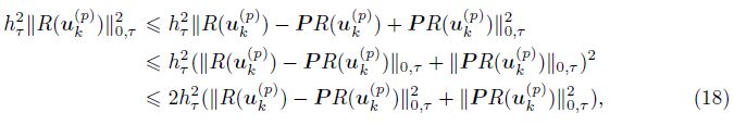
Using (10), the linearity of (·, ·)_τ , supp(B_τPR(u_k^(p) )) ⊂ τ, the Cauchy-Schwarz inequality, the definition of ║·║_{τ, 1},  (11), and the inverse inequatity, we have

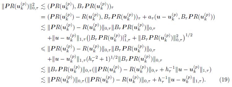
Notice that there is ║PR(u_k^(p) )║_{0, τ} on both sides of (19). We get

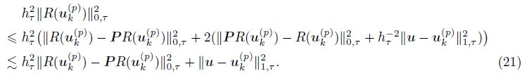
Substituting (20) into (18) and using (a + b)² ≤ 2(a² + b²), we have

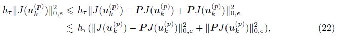
Secondly, we estimate h_τ║J(u_k^(p) )║_{0, e}².

By the triangular inequality and (a + b)2 6 2(a2 + b2), we get the following inequality:

where P is an L2-projection operator based on (P_p)².

Using (10), the linearity of (·, ·)_e, (16), supp(B_ePJ(u_k^(p) )) ⊂ Ω_e, and the Cauchy-Schwarz inequality, we have

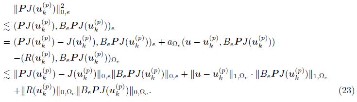
We obtain the following inequality by the inverse inequatity:

By substituting (24) into (23) and by (13) and (14), we get

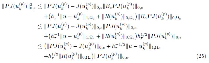
By getting rid of ║PR(u_k^(p) )║_{0, e} from both sides of (25), we obtain

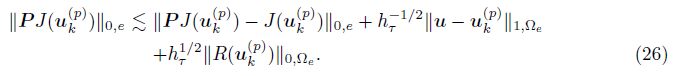
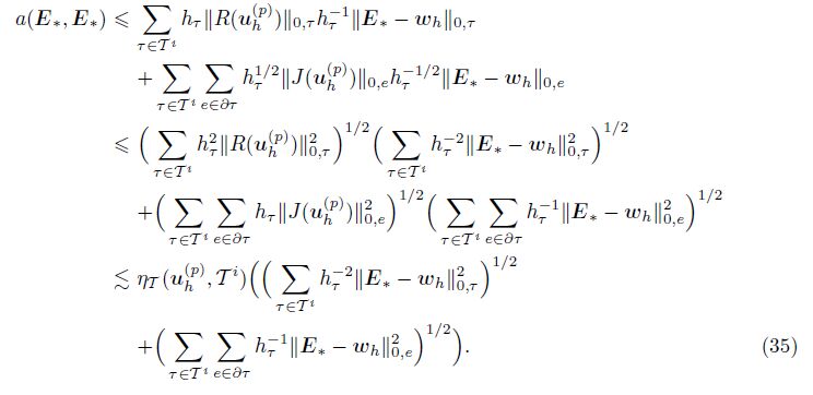
Combining (22) with (26) and using the inequality (a + b + c)² ≤ 3(a² + b² + c²) and the shape regularity of T_h, we get

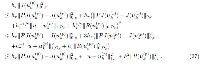
Combining (27) with (21), we have

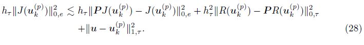
Using the definition of η₂(u_h^(p) , T_h), (21), and (28) and these definitions of O²(u_h^(p) , T_h) and ‖·‖_{1, Th}, we have

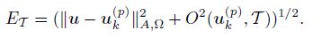
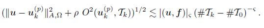
To prove the optimality of the AFEM, we need a localized upper bound for the distance between two nested solutions.

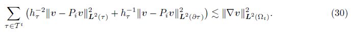
Lemma 5 (Localized upper bound) For any triangle grid T_k, T_k+1 ∈ C(T₀, T_k+1 is generated from T_k. Let D be the set of refined elements of T_k. Let u_k^(p) ∈ V_k^(p) and u_k+1^(p) ∈ V _k+1^(p) be the discrete solutions of (5) based on the grid T_k and T_k+1, respectively. Then, we have the following localized upper bound:

which depends on r, λ, μ, and the constant C₃ > 0 of the shape regularity of T₀.

Proof Let Ω_R := $\mathop \cup \limits_{\left\{ {\tau :\tau \in R} \right\}} $⊂ Ω be the union of refined elements, and denote by Ω_i (i =1, 2, · · · , J) the connected components of its interior. Let V(R) be the restriction of V_h^(p) to Ω_R. For any i ∈ {1, 2, · · · , J}, we define Tⁱ = {τ ∈ T : τ ⊂ $\bar \Omega $_i}, and let V (Tⁱ) be therestriction of V _h^(p) to Ω_i.

Let P_i : H¹(Ω_i) → V(Tⁱ) be the Scott-Zhang interpolation operator over the triangulation Tⁱ, and the following interpolation estimate holds true for all v ∈ H1(Ω_i):

Let E_∗ = u_h*^(p) - u_h^(p) ⊂ V _h*^(p). We construct wh by setting

Using (31), we get

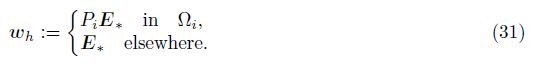
Using the nesting of spaces V _h^(p) ⊂ V _h*^(p), we thus obtain the Galerkin orthogonality,

Using (33), (32), the definition of E_∗, the linear property of a_τ(·, ·), (5), the definition of a(·, ·), the Green formulation, and the definition of operator L, we thus have

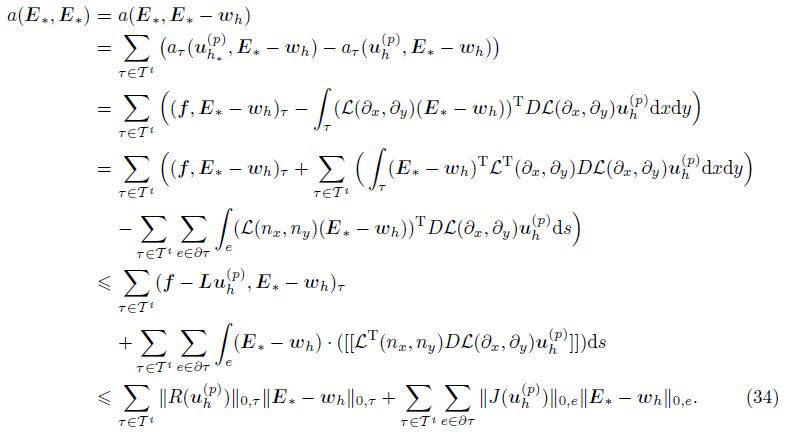
In the first and second terms of (34), we make them h ×h_τ^-1 and h_τ^1/2 ×h_τ^-1/2, respectively. Using the Cauchy-Swartz inequality and the definition of ηT (u_h^(p) , Tⁱ), we have

Using the inequality $\sqrt a $+ $\sqrt b $ ≤$\sqrt {2(a + b)} $, we have

By (30), we deduce that

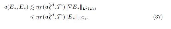
Using the coercivity of a(·, ·) and (36), we obtain

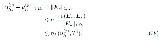
Squaring both sides of (38) and summing all i = 1, 2, · · · , J, we obtain

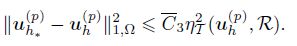
According to the norm equivalence, we thus have i2

which leads to (29).

We follow the recent framework developed by considering the total error^[15]

According to Theorem 1 of Ref. ^[17] (orthogonality), we deduce

Further, using (39) and the oscillation monotonicity (see Lemma 1), we obtain where T_∗ is a triangle grid through refining T .

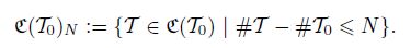
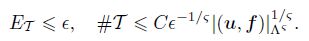
Now, we define an approximation class ${\Lambda _\varsigma }$ based on the total error. Let C(T_0N ⊂ C(T₀ be the set of all possible conforming triangle grids generated from T₀ with at most N elements more T₀,

For any ς > 0, the nonlinear approximation class ${\Lambda _\varsigma }$ can be defined as i6

Given N ≥ N₀ := #T₀, due to T ∈ C(T_0N generated from T₀, there exists an triangle grid T _N^∗ ∈ C(T_0N with # T _N^∗ = N and E_TN^*= €_N. We replace inf with min in the primitive definitions in Refs. ^[15] and ^[23].

According to Remark 5.1^[23], for any € > 0, we can choose a triangle grid T generated from T₀ with

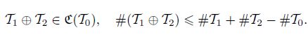
For any conforming mesh T₁, T₂ ∈ C(T₀), we define the following add mesh T₁ ⊕ T₂ by the form^[15]. The add mesh retains the following properties:

We can obtain a new triangle grid T∗ through refining T_k, and because of the convergence of total error, the total error of the new triangle grid is less than some given constant. We need to control the number of the new elements about the quasi-optimal.

Lemma 6 For some κ ∈ (0, 1), through refining T_k, we can obtain a new triangle grid T_∗ with

(i) E_T* ≤ κE_Tk ,

(ii) #T_* - #T_k ≤ C_KE_Tk^{-1/$\varsigma $}|(u, f)|_{${\Lambda _\varsigma }$}^{1/$\varsigma $}, where C_κ only depends on κ.

Using the definition of the oscillation, the finite element estimator, the triangle inequality, and the standard scaling argument, we get the following result.

Lemma 7 Let T_kh ∈ C(T₀. For any τ ∈ T_k and the finite element functions v_k^(p) , w_k^(p) ∈V _k^(p) , we have

where the constant C₄ only depends on the shape regularity of T₀, the constant λ, and μ.

Corollary 1 (Perturbation of oscillation) Let T , T_∗ ∈ C(T₀, and T∗ is a triangle grid through refining T . For all v_k^(p) ∈ V _h^(p) , v_k+1^(p) ∈ V _k+1^(p), we have

where the constant C₅ only depends on the constant C₄ of Lemma 7 and the shape regularity of the triangle grid T_k.

Proof Using (9), the nested mesh v_k^(p) ∈ V_h^(p) ⊂ V _k+1^(p), and Lemma 7 , for any τ ∈ T ∩T_∗, we have

We now sum over τ ∈ T_k ∩ T_k+1 to prove the assertion (40).

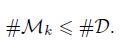
The key to relate the best mesh with the AFEM triangle grid is the fact that the procedure MARK selects the marked set M_k with the minimal cardinality. The following lemma will introduce the cardinality of M_k. Using the above lemmas, we can give the set of the marked elements with the mininal cardinality.

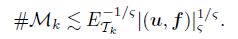
Lemma 8 (Cardinality of M_k) Let u be the solution of (4), and let {T_k}_k≥0 be the mesh sequence generated by the AFEM. Let M_k ⊂ T_k be the set of the marked elements with the mininal cardinality. If (u, f) ∈ ${\Lambda _\varsigma }$ , and the initial mesh T₀ satisfies a fineness assumption, for any ϑ ∈ (0, ϑ_∗) with ϑ_∗ =$\frac{{{C_2}}}{{1 + {C_3}(1 + 2{C_5})}}$ ) < 1, then the following estimate is true:

Proof Let κ := 2^-1(1 - ϑϑ_∗ ^-1) ∈ (0, 1), according to Lemma 6, there exists a triangle grid T_k+1 ∈ C(T₀ with the minimal elements number satisfying

Using Lemma 4, (41), and the definition ET_k and ET_k+1 , we have

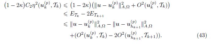
First, we discuss the error ‖u-u_k^(p) ‖_A², -‖u-u_hk+1^(p)‖_{A, Ω}² of (43). Using the orthogonality (see Theorem 1 of Ref. ^[17]) and the localized upper bound (Lemma 5), we have

where the subset D ⊂ T_k denotes the set of the marked elements.

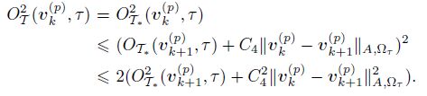
Then, we discuss the oscillation O2(u_k^(p) , T_k) - 2O2(u_hk+1^(p), T_k+1) of (43) by distinguishing the following two cases.

For any τ ∈ T_k\T_k+1, in view of (8), we have

For any τ ∈ T_k ∩ T_k+1, using Corollory 1 and Lemma 5, we have

Using (45) and (46), we obtain

Combining (43) with (44) and (47), we have

Dividing the constant 1 + C₃(1 + 2C₅) on both sides of the above equation and using the definition of κ and ϑ_∗, we get

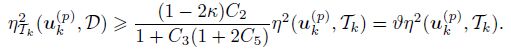
During the module MARK, we always choose the set M_k with

Then, we have

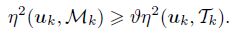
Due to the definition D and (42), we have

As a consequence of the previous estimates and the convergence of the AFEM, we obtain quasi optimality of the total error.

Theorem 2 (Quasi-optimal complexity) Given ϑ ∈ (0, ϑ_∗) with ϑ_∗ =$\frac{{{C_2}}}{{1 + {C_3}(1 + 2{C_5})}}$ < 1. Let u be the solution of (4), and let {u_k^(p) , T_k}_k≥0 be the sequence generated by the AFEM. Let (u, f) ∈ ${Lambda _\varsigma }$ , and let the bisection satisfy the assumptions (i) and (ii). Thus, we have

Proof Combining (7) and Lemma 8, we have

Using the global lower bound (17) and ρ < 1, we have

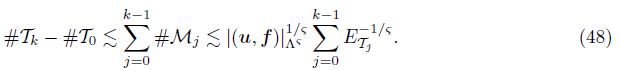
According to the convergence result (see Ref. ^[17]), for any j (0≤j≤k - 1), we get

Combine (49), (48), and (50). We obtain

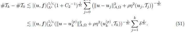
Using the global lower bound (17), we have

Since δ < 1, the geometric series$\sum\limits_{j - 1}^k {\delta \frac{j}{{{2_\varsigma }}}} $ is bounded by the constant S_ϑ = ${\delta ^{\frac{1}{{{2_\varsigma }}}}}{(1 - {\delta ^{\frac{1}{{{2_\varsigma }}}}})^{ - 1}}$, and combining (51) and (52), we obtain

By raising (53) to the sth power and reordering, we obtain the estimate for the error with C > 0 independent of ς.

4 Numerical experiments

In this section, we give two experiments to verify the theoretical result. During these experiments, we adopt the energy norm ‖·‖_AΩ, = a(·, ·)^{$\frac{1}{2}$} to do the error analysis, the modulus of elasticity E = 3 000 MPa, Poisson’s ratio ν = 0.3, and the error control constant e_tol = 10^-9.

During the following experiments, we use the linear and quadratic finite element methods to solve these corresponding discrete systems.

Example 1 Let Ω = [-1, 1]²\[0, 1]×[-1, 0], the proper vector function f and the boundary functions g and g_S are chosen to ensure the solution u = (u₁, u₂)^T, where

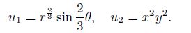
Figure 1 and 2 are the 15th and 20th refinement meshes, respectively. From these figures, we can see that the refinement elements are concentrated with singular of the solution u. In Fig. 3 and 4, we present two error curve figures about the errors of the solution u and the finite element solution u_k under the energy norm with the Döffler parameter ϑ = 0.1, 0.3, 0.5, respectively. In these figures, the abscissa value N_k represents the number of elements of the mesh T_k, and the ordinate value ‖u - u_k‖_{A, Ω} represents the energy norm of the error between the solution u and the finite element solution u_k. These straight lines with slope -$\frac{1}{2}$or -1 can be moved vertically.

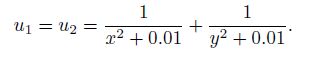
Example 2 Let Ω = [-1, 1]², and the proper vector function f and the boundary functions g, g_S are chosen to ensure the solution u = (u₁, u₂)^T, where

Using the same methods to solve the corresponding discrete systems of Example 2, we get the following results. Figure 5-8 are the experimental results about the above methods, respectively. In Fig. 5 and 6, we show the 15th and 16th refinement meshes. From these figures, we can see that the refinement elements are concentrated with singular of the solution u. In Fig. 7 and -8, we present two error curve figures about the errors of the solution u and the finite element solution u_k under the energy norm with the Döffler parameter ϑ = 0.1, 0.3, 0.5, respectively.

Example 3 Let Ω = ^{[-2, 2]2}, and the proper vector function f and the boundary functions g and g_S are chosen to ensure the solution u = (u₁, u₂)^T, where

Using the same methods to solve the corresponding discrete systems of Example 3, we get the following results. Figure 9-12 are the experiment results about the above methods, respectively. In Fig. 9 and 10, we show the 18th and 20th refinement meshes. From the two figures, we can see that the refinement elements are concentrated with singular of the solution. In Fig. 11 and 12, we present two error curve figures about the errors of the solution u and the finite element solution u_k under the energy norm with the Döffler parameter ϑ = 0.1, 0.3, 0.5, respectively.

From Fig. 3, 4, 7, 8, 11, and 12, we confirm that the adaptive finite element algorithm (Algorithm 1) is quasi-optimal. That is, these error curves decline along with the number of the increasing triangle elements. For the linear and quadratic finite element methods, the error curves of ‖u - u_k‖_{A, Ω}, are almost parallel with the straight lines of the slopes -$\frac{1}{2}$ and -1 separately. Moreover, we can get the conclusion that Algorithm 1 is robust with the Döffler parameter ϑ ∈ (0.1, 0.5).

5 Conclusions

In the paper, we rigorously prove that the adaptive finite method is quasi-optimal and verify this conclusion by some experiments for linear elasticity problems in two dimensions. Similarly, we can get the resemble conclusion for linear elasticity problems in three dimensions.