 2016, Vol. 37
Article Information
- Xi CHEN, Ying DAI. 2016.
- Differential transform method for solving Richards' equation
- Appl. Math. Mech. -Engl. Ed., 37(2): 169-180
- http://dx.doi.org/10.1007/s10483-016-2023-8
Article History
- Received Feb. 9, 2015;
- in final form Jul. 7, 2015


The Richards’ equation, which quantitatively describes the process of fluid infiltrating the porous medium such as soil, concrete, etc., is a nonlinear partial differential equation (PDE) about the saturation of unsaturated porous media in most cases[1, 2, 3, 4]. It is given as
Several analytical and numerical solutions for the Richards’ equation with the Brooks-Corey model were obtained by many researchers, such as Bruce and Klute[12], Parlange[13], Prasad and Romkens[14], Witelski[15], Lockington et al.[3], Barry et al.[16], and Omidvar et al.[11]. In these studies, some have obtained the implicit solutions of Richards’ equation without the hydraulic conductivity K(S)[1, 3, 12, 13, 14], and others based on wetting front propagation, have derived the traveling wave approximate solution[15]. Recently, Omidvar et al.[11] used the differential transform method (DTM) and the homotopy perturbation method (HPM) to obtain the analytical solution of the Brooks-Corey model with 1-2 orders power series types.
Learning from the studies above, the DTM is found to be robust in finding solutions of Richards’ equation. This paper tries to use the DTM to search the analytical solution of Brooks-Corey model with the high order power series type, which is usually used to describe the unsaturated fluid flow in concrete or soil[1, 17].t
Nevertheless, there are two problems in the DTM. One is that the convergence speed is very slow as the calculated point is away from the convergence center. For example, some- times it needs about 400 approximations to ensure accuracy in calculating the Brooks-Corey model[11]. The other is that the DTM, which is based on Taylor’s theorem, is usually hard to solve the discontinuous solution problem, such as discontinuity between initial and boundary conditions[3].
For the problems of the DTM above, the solution of extension of Heaslet-Alksne technique[1] is used as an intermediate variable to accelerate the convergence speed of the DTM. For dealing with the discontinuous solution problem, the Boltzmann variable φ=$\frac{x}{{\sqrt t }}$ and a tiny time point △t are introduced in two forms K(S) = 0, and K(S)≠0, respectively, to change the Richards’ equation into an ordinary differential equation (ODE) instead of using the wave variable from Alquran[18] in this paper. In the end, two numerical examples are given to show the accuracy of the presented approach.
2 Brooks-Corey model and definite conditionsAccording to Parlange et al.[1] and Witelski[4], the functional relationship between D(S), K(S), and S is presented as

From the works of Lockington et al.[3] and Witelski[4], the initial condition of Eq. (1) could be expressed as a constant moisture concentration


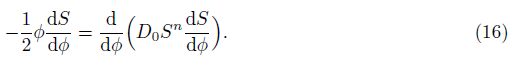
The DTM was presented in 1986 by Zhou[19], who used Taylor series for the solution of linear and nonlinear differential equations in the form of polynomial. From the pioneer studies on the DTM conducted by several researchers[20, 21, 22, 23, 24, 25, 26, 27, 28, 29, 30, 31], the basic concept of the DTM is that each function S(x) in the governing equation can be expressed as
Theorem 1 If S(x) = S1(x) ± S2(x), then Y (n) = Y1(n) ± Y2(n).
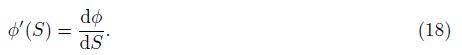
Theorem 2 If S(x) = cS1(x), then Y (n) = cY1(n), where c is a constant.
Theorem 3 If S(x) = $\frac{{{d^k}{S_1}(x)}}{{d{x^k}}}$, then Y (x) = $\frac{{(n + k)!}}{{n!}}$ Y1(n + k).
Theorem 4 If S(x) = S1(x)S2(x), then Y (n) =$\sum\limits_{{n_1} = 0}^n {} $ Y1(n1)Y2(n - n1).
According to Alquran[18], an intermediate variable ξ is introduced to change the PDE into an ODE. Then, the DTM can be applied to the resulting ODE through the following steps.
(i) Construct an intermediate variable ξ = ξ(x, t) such that


(iii)φ(ξ) in Eq. (9) could be expressed as
(iv) Apply the DTM to Eq. (11), and calculate U(n) as
(v) The approximate solution is
There are two forms for Richards’ equation, namely, the horizontal infiltration form K(S) ≠ 0 and the vertical infiltration form K(S)≠0 in Eq. (1). In this section, we shall discuss them, respectively.
Case 1 K(S) = 0
Due to K(S) = 0, Eq. (1) can be expressed
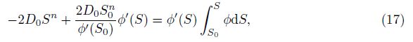
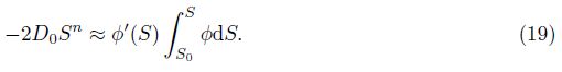


From Eqs. (20)-(24), we can find that the discontinuous problem between the initial condi- tion (4) and the boundary condition (5) can be solved by the Boltzmann variable φ, and the discontinuous solution problem (1) with initial and boundary conditions (4)-(6) is changed into the continuous solution problem (19) with boundary conditions (23) and (24). According to the extension of the Heaslet-Alksne technique[1] and the step (i) in Section 3, we construct an intermediate variable ξ as follows:

The new boundary conditions (23) and (24) may be changed into


By introducing the intermediate variable ξ, Eq. (19) is


Substituting Eq. (26) into Eq. (30), we obtain
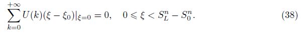
Based on the initial terms Y1(0) and Y2(0) and the differential transformation formula (38), we could obtain U(k) in Eq. (26) by calculating the parametersW(k-1), Y1(i), and Y2(k-1-i) in Eqs. (32)-(35) term by term.
Case 2 K(S) ≠ 0
Because K(S) ≠ 0, the discontinuous problem between the initial condition (4) and the boundary condition (5) can not be solved by the Boltzmann variable φ. At this time, we still suppose that the saturation S could be expressed as
Instead of solving the differential transformations of the initial condition (4) and the bound- ary conditions (5) and (6) directly, we choose a tiny time point △t → 0, substitute t = △t into Eq. (1), and yield


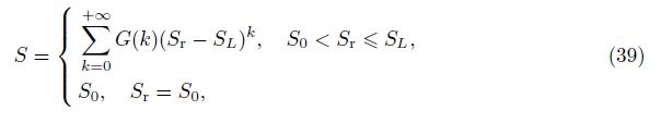
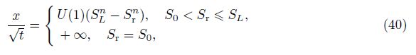
According to Eqs. (39) and (40), when t → 0 or x → +∞, we have Sr = S0 and S = S0, which indicates that the initial condition (4) and the boundary condition (6) are naturally satisfied. On the other hand, when x = 0, we have Sr = SL, which means that the boundary condition (5) is

According to Theorem 1 in Section 3, the transformation form of K(S)≠0 in Eq. (42) is


Substituting Eq. (39) into Eq. (45), we obtain

Based on the initiazl terms W1(0), F1(0), F2(0), F3(0), F4(0), and F5(0), and Eq. (62), we could obtain G(k) in Eq. (39) (K(S)≠0) by calculating the parameters W1(k -1), W2(k -1), W3(k - 1), and W4(k - 1) in Eq. (46) term by term.
5 Numerical simulationIn this section, we apply the method in Section 4 to study two examples.
Example 1 D(S) = 0.138 243S8, K(S) = 0, S0 = 0, SL = 1[3].
According to Eq. (25) in the case 1, the intermediate variable ξ is
By choosing k = 1, 2, 3, respectively, we obtain U(k) in S ∈ (0, 1] as follows:
k = 1, U(0) = 0, U(1) = 0.197 182;
k = 2, U(0) = 0, U(1) = 0.203 251, U(2) = -0.012 703;
k = 3, U(0) = 0, U(1) = 0.202 618, U(2) = -0.012 663 6, U(3) = 0.001 320 735.
Substituting U(k) into Eq. (64), we obtain 1-3 orders approximation solutions as follows:
1 order approximation solution
2 orders approximation solution

3 orders approximation solution

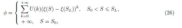
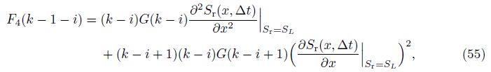
Compared with the finite element method (FEM) in the space coordinate x varying from 0 to 0.25mm, which is divided into 280 units and calculated for results with saturation S in t = 1min as the exact solution, the present method shows the results of 1-3 orders approximations of Eqs. (65)-(67) in Fig. 1. The results of saturation S obtained from Eq. (67) are compared with the results from the FEM in Table 1.

|
| Fig. 1 Results of saturation S obtained from FEM and present method in D(S) = 0.138 243S8 |

From Fig. 1, it can be seen that the saturation S decreases from 1 to 0 as the Boltzmann variable φ increases. Due to the effect of hydraulic diffusivity D(S), the saturation S decreases very fast from 0.7 to 0.1 when φ is changed from 0.18 to 0.19mm·min-$\frac{1}{2}$ . The solutions of the present method are closer to the exact solutions as the order k increases from 1 to 3 in Fig. 1.
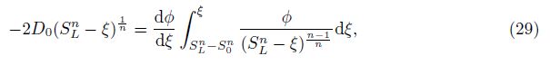
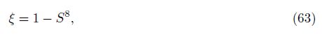
In Table 1, the results of the 3 orders approximation solution are very close to the results of the FEM. The maximum relative error value of present method is -0.227 56% in S = 0.4 for the 3 orders approximation solution. In the meantime, using the DTM without introducing the intermediate variable ξ, we obtain the 1-3 orders approximate solutions by solving Eq. (19) and boundary conditions (23) and (24) with D(S) = 0.138 243S8, K(S) = 0, S0 = 0, and SL = 1. The corresponding results are shown in Fig. 2.

|
| Fig. 2 Results of saturation S obtained from FEM and DTM without intermediate variable in D(S) =0.138 243S8 |
Compared with Fig. 1, the results of 1-3 orders approximate solutions without the interme- diate variable in Fig. 2 are more difficult to converge to the results obtained from the FEM.
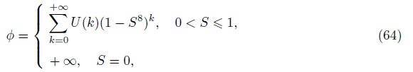
Example 2 D(S) = 12 250.497 546 61S6, K(S) = 6 078.024 95S11, SL = 0.36, and S0 = 0.042 84[28].
According to the case 1 and Eq. (40), the 1 order approximation solution of K(S) = 0 is
From the case 2, supposing the 1 order approximation solution of Sr as the intermediate variable, the tiny time point △t = 1 × 10⁻⁶s and choosing k = 1, 2, 3 in Eq. (69), respectively, we obtain G(k) in S ∈ (0.042 84, 0.36] as follows:
Substituting G(k) into Eq. (69), we obtain that 1-3 orders approximation solutions as follows:
1 order approximation solution

2 orders approximation solution

3 orders approximation solution
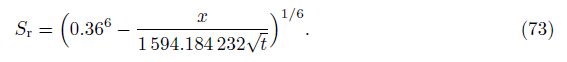
According to Eq. (69), the intermediate variable Sr in Eqs. (71)-(73) is

|
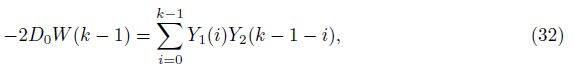
| Fig. 3 Results of S obtained from FEM and approximation solutions of different orders (t = 1 s) |

According to Fig. 3, the saturation S decreases from 0.36 to 0.042 84 when the infiltration depth x increases. The solutions of the present method are closer to the exact solutions as the order k increases from 1 to 3 gradually. In Table 2, the differences of results between the present method and the FEM are small. The maximum relative error value of the present method is -3.454 29% when x = 3.42mm in the 3 orders approximation solution.
6 ConclusionIn this paper, we have applied the DTM for solving the Richards’ equation with the Brooks- Corey model. By introducing an intermediate variable ξ into the governing differential equation, we successfully increase the convergence rate of solutions with the DTM and derive the 1-3 or- ders approximate solutions of K(S) = 0. For the form of K(S)≠0, we solve the discontinuous solution problem by introducing a tiny time point △t and do the differential transformation based on the corresponding 1-3 orders approximate solutions of K(S) = 0 at the time t = △t. The presented examples demonstrate the accuracy of the present solution by comparing the present results with the results obtained from the FEM.
| [1] | Parlange, M. B., Prasad, S. N., Parlange, J. Y., and Romkens, M. J. M. Extension of the Heaslet-Alksne technique to arbitrary soil water diffusivities. Water Resources Research, 28, 2793-2797(1992) |
| [2] | Forsyth, P. A., Wu, Y. S., and Pruess, K. Robust numerical methods for saturated-unsaturated flow with dry initial conditions in heterogeneous media. Advances in Water Resources, 18, 25-38(1995) |
| [3] | Lockington, D., Parlange, J. Y., and Dux, P. Sorptivity and the estimation of water penetration into unsaturated concrete. Materials and Structures/Materiaux Et Constructions, 32, 342-347(1999) |
| [4] | Witelski, T. P. Motion of wetting fronts moving into partially pre-wet soil. Advances in Water Resources, 28, 1131-1141(2005) |
| [5] | Fredlund, D. G. and Anqing, X. Equations for soil-water characteristic curve. Canadian Geotech-nical Journal, 31, 521-532(1994) |
| [6] | Campbell, D. S. A simple method for determining unsaturated conductivity from moisture reten-tion date. Soil Science, 117, 311-314(1974) |
| [7] | Brooks, R. H. and Corey, T. Hydraulic Properties of Porous Media, Colorado State University, Colorado (1964) |
| [8] | Gardner, W. R., Hiller, D., and Benyamint, Y. Post irrigation movement of soil water.: redis-tribution. Water Resources Research, 6, 851-861(1970) |
| [9] | Van Genuchten, M. T. A closed-form equation for predicting the hydraulic conductivity of unsat-urated soils. Soil Science Society of America Journal, 44, 892-898(1980) |
| [10] | Russo, D. Determining soil hydraulic properties by parameter estimation: on the selection of a model for the hydraulic properties. Water Resource Research, 24, 453-459(1988) |
| [11] | Omidvar, M., Barari, A., Momeni, M., and Ganji, D. D. New class of solutions for water infiltration problems in unsaturated soils. Geomechanics and Geoengineering: An International Journal, 5, 127-135(2010) |
| [12] | Bruce, R. R. and Klute, A. The measurement of soil moisture diffusivity. Soil Science Society of America Journal, 20, 458-462(1956) |
| [13] | Parlange, J. Y. Theory of waterm ovementin soils I: one dimensional absorption. Soil Science, 111, 134-137(1971) |
| [14] | Prasad, S. N. and Romkens, M. J. M. An approximate integral solution of vertical infiltration under changing boundary condition. Water Resource Research, 18, 1022-1028(1982) |
| [15] | Witelski, T. P. Perturbation analysis for wetting fronts in Richards' equation. Transport in Porous Media, 27, 121-134(1997) |
| [16] | Barry, D. A., Parlange, J. Y., Li, L., Prommer, H., Cunningham, C. J., and Stagnitti, F. Analyt-ical approximations for real values of the Lambert W-function. Mathematics and Computers in Simulation, 53, 95-103(2000) |
| [17] | Hall, C., Hoff, W. D., and Wilson, M. A. Effect of non-sorptive inclusions on capillary absorption by a porous material. Journal of Physics D: Applied Physics, 26, 31-34(1993) |
| [18] | Alquran, M. T. Applying differential transform method to nonlinear partial differential equations: a modified approach. Applications and Applied Mathematics, 7, 155-163(2012) |
| [19] | Zhou, J. K. Differential Transform and Its Applications for Electrical Circuits (in Chinese), Huazhong University Press, Wuhan (1986) |
| [20] | Chen, C. K. and Ho, S. H. Application of differential transformation to eigenvalue problems. Applied Mathematics and Computation, 79, 173-188(1996) |
| [21] | Chen, C. K. and Ho, S. H. Solving partial differential equations by two-dimensional differential transform method. Applied Mathematics and Computation, 106, 171-179(1999) |
| [22] | Ayaz, F. On the two-dimensional differential transform method. Applied Mathematics and Com-putation, 143, 361-374(2003) |
| [23] | Su, X. H. and Zheng, L. C. Approximate solutions to MHD Falkner-Skan flow over perme-able wall. Applied Mathematics and Mechanics (English Edition), 32(4), 401-408(2011) DOI 10.1007/s10483-011-1425-9 |
| [24] | Zou, L., Wang, Z., Zong, Z., Zou, D. Y., and Zhang, S. Solving shock wave with discontinuity by enhanced differential transform method (EDTM). Applied Mathematics and Mechanics (English Edition), 33(12), 1569-1582(2012) DOI 10.1007/s10483-012-1644-9 |
| [25] | Khader, M. M. and Megahed, A. M. Differential transformation method for studying flow and heat transfer due to stretching sheet embedded in porous medium with variable thickness, vari-able thermal conductivity, and thermal radiation. Applied Mathematics and Mechanics (English Edition), 35(11), 1387-1400(2014) DOI 10.1007/s10483-014-1870-7 |
| [26] | Arikoglu, A. and Ozkol, I. Solution of difference equations by using differential transform method. Applied Mathematics and Computation, 174, 1216-1228(2006) |
| [27] | Arikoglu, A. I. Solution of boundary value problems for integro-differential equations by using differential transform method. Applied Mathematics and Computation, 168(2), 1145-1158(2005) |
| [28] | Dickinson, R. E., Henderson-Sellers, A., and Kennedy, P. J. Biosphere atmosphere transfer scheme (BATS) for NCAR community climate model. NCAR Technical Note, NCAR/TN-275+STR (1986) |
| [29] | Mosayebidorcheh, S. Analytical investigation of the micropolar flow through a porous channel with changing walls. Journal of Molecular Liquids, 196, 113-119(2014) |
| [30] | Mosayebidorcheh, S. Solution of the boundary layer equation of the power-law pseudoplastic fluid using differential transform method. Mathematical Problems in Engineering, 2013, 685454(2013) |
| [31] | Mosayebidorcheh, S., Ganji, D. D., and Farzinpoor, M. Approximate solution of the nonlinear heat transfer equation of a fin with the power-law temperature-dependent thermal conductivity and heat transfer coefficient. Propulsion and Power Research, 3, 41-47(2014) |