 2016, Vol. 37
Article Information
- Sicheng WANG, Sixun HUANG. 2016.
- Sufficient conditions of Rayleigh-Taylor stability and instability in equatorial ionosphere
- Appl. Math. Mech. -Engl. Ed., 37(2): 181-192
- http://dx.doi.org/10.1007/s10483-016-2022-8
Article History
- Received Apr. 17, 2015;
- in final form Jul. 21, 2015


2. State Key Laboratory of Satellite Ocean Environment Dynamics, Second Institute of Oceanography, State Oceanic Administration, Hangzhou 310012, China
In the past over 70 years, considerable efforts have been taken to describe and explain the equatorial plasma bubbles (EPBs) phenomena from both an experimental and a theoret- ical viewpoints. It is now generally believed that the physical mechanism responsible for the growth of EPBs is Rayleigh-Taylor (R-T) instability[1, 2, 3]. The R-T instability is excited in the bottomside F region and evolves into a plasma bubble that penetrates the F peak to the topside F region. More recently, with the continuing installation of, and our increased dependence on, global navigation satellite systems, such as the American Global Positioning System (GP(S)), the European Galileo, the Chinese COMPA(S)S/Beidou, the Russian Global Navigation Satel- lite System, and the Japanese Quasi-Zenith Satellite System constellations, the importance of understanding and predicting the occurrence of EPBs has significantly increased[4]. EPBs oc- currence has complex temporal and spatial variations. To better forecast the generation and development of EPBs, it is necessary to study the R-T instability in the equatorial ionosphere.
Hydrodynamic instability is one of the important topics in the fields such as fluid mechan- ics, plasma dynamics, and atmospheric dynamics. The linear instability theory based on the normal mode method has much more achievements in the hydrodynamic instability research. Rayleigh[5] deduced the linear instability necessary condition for the parallel shear flow of invis- cid fluid, which is the well-known Rayleigh criterion. Fjortoft[6] extended the Rayleigh criterion, but the sufficient condition has not been derived. Howard[7] presented the semicircle theorem, that is, all eigenvalues of the instability models must locate in a given semicircle. In the recent years, researchers all around the world have made significant contributions to hydrodynamic instability studies, including linear, weakly nonlinear, and nonlinear hydrodynamic instability studies[8, 9, 10, 11, 12, 13, 14].
In the present study, the R-T stability and instability sufficient conditions in the equatorial F region are deduced based on the electron/ions continuity equations, momentum equations, and the current continuity equation[15, 16, 17, 18, 19, 20, 21, 22, 23, 24, 25]. First, small perturbation linear equations that are vari- able coefficient partial differential equations are obtained. Second, these equations are changed to the eigenvalue equations by the normal mode method, and the sufficient conditions of R-T stability and instability are derived by the variational approach. Last, an approximate numer- ical method of solving systematic eigenvalues is introduced, and a modified numerical model of the development of EPBs is used to validate the sufficient conditions.
2 Basic theoryUsing a geomagnetic west, vertically up and geomagnetically north Cartesian coordinate system (x, y, z). The geomagnetic field B is in the z-direction. In the F region, O+ is the dom- inant ion, and other ion species are neglected. The electrodynamics of the nighttime equatorial ionosphere can be expressed by the ion/electron continuity equations, momentum equations, and the current continuity equation as follows[26, 27]:


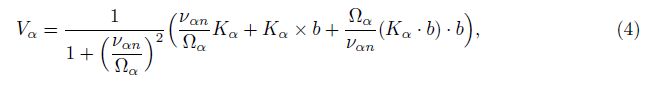


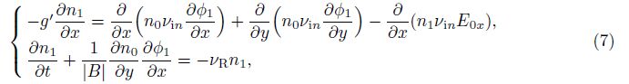
Equations (1) and (2) are now perturbed and linearized by using n = n0+n1, E = E0+E1 = -∇ψ0 - ∇ψ1, and '0 is the zeroth-order electric potential. Supposing that υin, n0 and υR are the functions of the altitude (y), and neglecting any second-order perturbation terms, small perturbation linear equations can be readily obtained
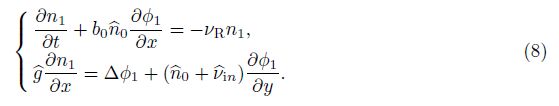
To study the electrostatic instability of (8) in the presence of a vertical zeroth-order den- sity gradient, we can write the perturbed electric potential and the plasma density as n1 = N(y) exp[iα(x - γ t)] and φ1 = Φ(y) exp[iα(x - γ t)], respectively, where N(y) and Φ(y) are the eigenfunctions, α is the wave number, γ= γr + iγi is the eigenvalue, and γr and γi are the real and imaginary parts, respectively. Substituting n1 and φ1 into (8) yields
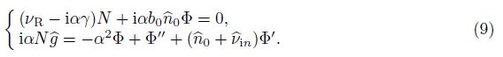
Using the local approximation α≫($\hat n$0+$\hat \nu $in)[20, 30, 31], the term ($\hat n$0+$\hat \nu $in)Φ′ in (9) is neglected. We have


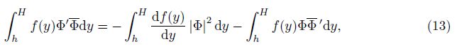
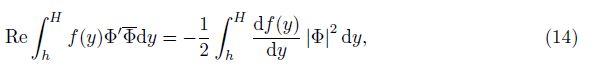
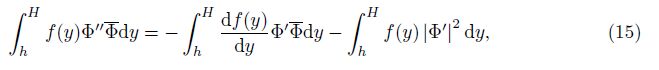
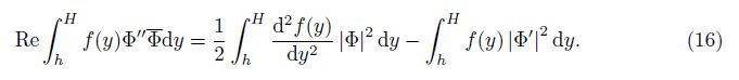
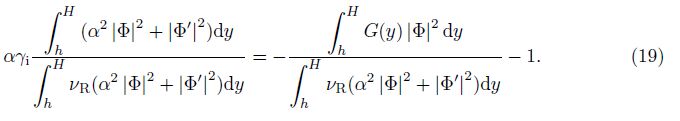
Equation (11) is similar to the Orr-Sommerfeld (O-S) equation in fluid dynamics at the first glance, but it has some differences in the first brackets. The differences can make the necessary condition derived in the fluid dynamics while the sufficient conditions are derived here. (11) is multiplied by $\bar \Phi $ ($\bar \Phi $ is the complex conjugate function of Φ), and the resulting expression is integrated with respect to y over the interval (h, H) with the boundary condition Φ(h) = Φ(H) = 0, which leads to


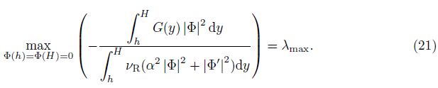
Let
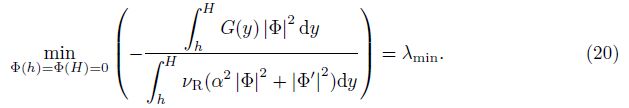
Similarly, let max
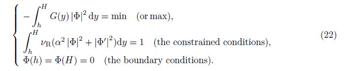
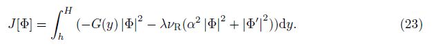
We introduce the functional J[Φ] as
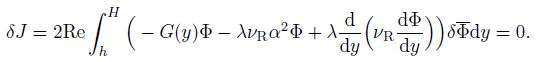
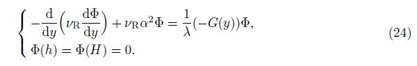
Then, the functional extreme value problems can be changed to the eigenvalue problems of the second-order differential equation, considering that δ$\bar \Phi $ is arbitrary, i.e.,
The eigenvalues reflect the systematic and comprehensive R-T instability and stability of the whole equatorial ionosphere altitude, rather than the R-T instability and stability of the specific ionosphere altitude or parameter. For eigenvalue problems, many methods and theories have been put forward. Here, we use an approximate method to estimate the systematic eigenvalues.
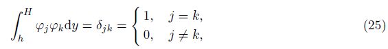
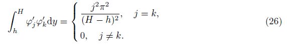
4 Approximate numerical calculation methodChoose the basis function ψj (y)=$\sqrt {\frac{2}{{H - h}}} $sin $\frac{{j\pi (y - h)}}{{H - h}}$ in the L2(h, H) space, which satisfies the following orthogonal relations:
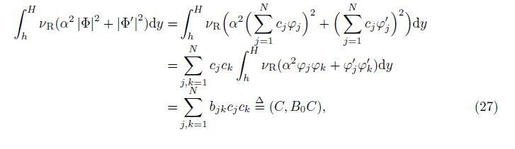

Then, (22) can be simplified to the following equations:
Introduce J[C] as

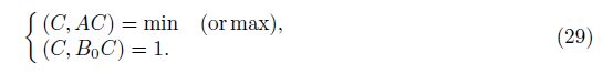
To get the minimum or maximum values, the first-order variation of J[C] shall be equal to zero, i.e.,

Since δ

If the eigenvalues of AC = λB0C are λ1≤λ2≤· · ·≤λN, λ1 is the minimum eigenvalue, and λN is the maximum eigenvalue. The ionosphere is R-T unstable when λ1 > 1, and the ionosphere is R-T stable when λN < 1.
5 Validation and discussionTo validate the sufficient conditions, some numerical experiments are performed in the follow- ing. In the numerical calculations, thermospheric quantities are obtained from the NRLM(S)I(S)E- 00 model[32], ionospheric parameters are from the 2007 International Reference Ionosphere (IRI- 2007) model[33]. The initial ambient electron density profile is superimposed on each contour figure for references, and the altitude ranges from 250 km to 450 km with the electron density peak altitude (hmF2) at ∼375 km. To make G(y) have the same sign, we take h as 250 km and H as 375 km. For simplicity, the magnetic field strength is regarded as uniform (3×10⁻⁵ T) in the simulation, and the horizontal electric field strength is supposed to be altitudinal uniformity in the initial background ionosphere.
Simulation 1 We just change the horizontal electric field strength, and other parameters are kept the same. The disturbance wave number is 1/km (the wavelength is ∼6 km), and the neutral wind velocity is zero. The minimum and maximum systematic eigenvalues versus the horizontal electric field strength are shown in Fig. 1. The unstable area derived from the sufficient condition is marked in white, and the stable area is in dark. The unstable area is located at the large eastward electric field strength regime. When the eastward electric field is present, the plasma can be lifted under the action of E × B, which steepens the electron alti- tudinal gradient further, and is beneficial to the development of R-T instability. The westward electric field can suppress the electron altitudinal gradient below the peak altitude, which is not conducive to the R-T instability.
Ossakow et al.[15] have set up the basic equations of the development of EPBs in the equa- torial ionosphere, including the effects of neutral wind and electric field. Huba et al.[26] showed that the R-T instability is not damped by recombination in the F region, and there is no source term υRn0 to maintain the electron density at the value n0 in the nighttime. Therefore, the models of EPBs development can be expressed as follows:


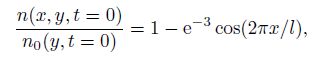
Among many previous works[15, 29, 31], superimposed on the background-density at t = 0 was a cosine-like perturbation of the form

|
| Fig. 1 Minimum (solid line) and maximum (dashed line) systematic eigenvalues versus horizontal electric field strength. Shading with different colors is used to show unstable area (white), stable area (dark), and uncertain area (light dark) derived from sufficient conditions. Note that westward direction is positive |
Case 1 Figure 2 shows the isodensity contours at different moments with l = 6 km initial perturbation, and the east-west extent is 15 km. The horizontal electric field strength is -2.0× 10⁻³ V/m. The initial disturbance amplitude is 5%. The white dashed line is the ambient electron density profile at the time t without the initial disturbance. Due to the recombination effects, the ambient electron density decreases gradually, especially in the bottomside F region. At 3 000 s (see Fig. 2(a)), the plasma bubble is quite obvious, and the maximum electron depletion is ∼80%. At 6 000 s, the plasma bubble has penetrated the peak altitude with an innermost depletion contour of ∼100% (see Fig. 2(d)). We also note that the other electron depletions in the wings are formed. The given ionosphere is R-T unstable, which is in accord with the conclusions derived in Fig. 1.

|
| Fig. 2 Contours of electron isodensity (105 el/cm3) at different moments with l = 6 km initial perturbation. (a), (b), (c) and (d) are at 3 000 s, 4 000 s, 5 000 s and 6 000 s with 5% amplitude initial disturbance, respectively. Black solid line is initial ambient electron density profile, and white solid line is electron density profile at time t without initial perturbation. Those two profiles in figure are normalized by initial NmF2 |
With the 0.5% initial perturbation, the bubble has been clearly formed in the bottomside F region, and the maximum electron depletion is ∼60% at 3 000 s (see Fig. 3(a)). The bubble has penetrated the F peak at 6 000 s (see Fig. 3(d)). When the ionosphere is R-T unstable, even the smaller amplitude initial perturbation (such as 0.5%) can trigger the ionospheric R-T instability and form EPBs.

|
| Fig. 3 Same as Fig. 2, but for 0.5% initial disturbance |
Case 2 When the horizontal electric field strength is E0x = 4 × 10⁻⁴ V/m, the ionosphere is R-T stable according to the sufficient condition. Figure 4 exhibits contour plots of electron density at 300 s and 3 000 s with l = 6 km initial perturbation. At 300 s, a cosine-like perturbation can be clearly found on the bottomside electron density with the 5% (see Fig. 4(a)) and 10% (see Fig. 4(c)) amplitude initial disturbances. It is not obvious that the electron depletion and enhancement at 3 000 s are under 5% initial perturbation conditions. The initial perturbations gradually become weakened, and the plasma bubble is difficult to grow and reach the topside F region. With the 10% initial perturbation (see Fig. 4(d)), no obvious electron depletion and enhancement exists. The initial perturbation gradually tends to be stabilized and is difficult to develop. When the ionosphere is R-T stable, even larger amplitude (such as 10%) initial perturbations cannot initiate the ionospheric R-T instability.

|
| Fig. 4 Contours of electron isodensity (105 el/cm3) after l = 6 km initial perturbation. (a) and (b) are at 300 s and 3 000 s with 5% initial disturbance, while (c) and (d) are at 300 s and 3 000 s with 10% initial disturbance, respectively. Black solid line is initial ambient electron density profile, and white solid line is electron density profile at time t without initial disturbance. Those two profiles in figure are normalized by initial NmF2 |
The EPBs can be initiated or suppressed when the systematic eigenvalues are in the range of λmin <1 and λmax >1 (marked in light dark in Fig. 1), that is, the ionosphere may be R-T unstable or stable in this eigenvalue extent, the corresponding figures of the development of EPBs are not shown here.
Simulation 2 We just change the zonal and vertical wind velocities, respectively, and other parameters are kept the same. The electric field strength is E0x = -6 × 10⁻⁴ V/m, and the wave number is 1/km. The minimum and maximum systematic eigenvalues are plotted versus the zonal wind velocity (a) and vertical wind velocity (b) in Fig. 5. The minimum systematic eigenvalues increase with the eastward wind velocity. According to the sufficient condition, the eastward wind is conducive to the development of R-T instability. In the evening sector, the horizontal pressure gradient across the terminator produces large thermospheric eastward zonal neutral winds. The equatorial zonal neutral winds interact with Earth’s magnetic field resulting in a vertical polarized electric field. At nighttime, E region plasma densities rapidly decay, the E region dynamo becomes negligible, and the F region dynamo dominates the nighttime plasma drifts[2]. Under such conditions, the neutral and ionized portions of the atmosphere at F region altitudes move eastward at the same speed. Additionally, the eastward neutral wind at the equator may explain the phenomena that the upper portions of bubbles will take on a westward tilt, while the lower portions will tilt eastward, giving rise to the ‘fishtails’ and ‘Cs’ observed by coherent backscatter radar measurements of field-aligned small-scale irregularities[34]. Cha- pagain et al.[35] showed that the nighttime and night-to-night variations in the zonal neutral winds, equatorial plasma bubble velocities, and plasma drifts were well correlated. Kudeki et al.[36] presented experimental evidence and modeling results which indicated that the eastward thermospheric wind was the primary controlling factor of equatorial spread-F (E(S)F) initiation in the post-sunset ionosphere.

|
| Fig. 5 Minimum (solid line) and maximum (dashed line) systematic eigenvalues versus zonal (a) and vertical (b) wind velocity under simulation 2 ionosphere conditions. Shading with different colors is used to show unstable area (dark) and uncertain area (light dark) derived from sufficient conditions. Note that vertical scale is logarithmic, and westward/upward directions are positive |
Sekar and Raghavarao[37] with the linear theory, and Raghavarao et al.[38] with the nonlinear numerical modeling, suggested that vertical downward (upward) winds have the potential to cause (inhibit) the ESF/bubble phenomenon. Sekar et al.[39] hypothesized that the variability in the occurrence characteristic of ESF was in connection with the possible day-to-day variability of vertical winds. Raghavarao et al.[40] showed evidence for the presence of downward winds collocated with irregularities in electric fields and plasma densities as revealed by a unique combination of highly accurate measurements with instruments onboard DE-2 satellite. From Fig. 5(b), it can be seen that the minimum systematic eigenvalues increase with the downward wind velocity, that is, the downward wind is beneficial to the development of R-T instability. The conclusion derived from the sufficient condition is consistent with the experimental and modeling results mentioned above.
6 ConclusionSufficient conditions of the R-T stability and instability in the equatorial ionosphere are preliminarily derived as follows: if the minimum systematic eigenvalue is greater than one, the ionosphere is R-T unstable, while if the maximum systematic eigenvalue is less than one, the ionosphere is R-T stable. To validate the sufficient conditions, we design some numerical experiments under different ionospheric parameters conditions. When the minimum systematic eigenvalue is greater than one, the plasma bubble arising from the initial perturbation can develop rapidly and penetrate the peak altitude, indicating that the ionosphere is R-T unstable. While the maximum systematic eigenvalue is less than one, the initial disturbance is difficult to grow and tends to be stabilized gradually, indicating that the ionosphere is R-T stable. The numerically experimental results show that our sufficient conditions are reasonable.
Sufficient conditions are deduced under the assumption of α≫($\hat n$0+$\hat \nu $in). In general, the scales of $\hat n$0 and $\hat \nu $in are both ∼10-2/km, and therefore the sufficient conditions are suitable to the initial perturbation of small wavelength. However, observations show that the large scale initial perturbation (∼102 km) can also cause the occurrence of EPBs[41]. How to take out the precondition α ≫ ($\hat n$0 + $\hat \nu $in) is the future work. Moreover, when the systematic eigenvalues are in the range of λmin < 1 and λmax > 1, the ionosphere can be R-T stable or unstable, which needs further study.
| [1] | Woodman, R. F. Spread F-an old equatorial aeronomy problem finally resolved? Annales Geo-physicae, 27, 1915-1934(2009) |
| [2] | Kelley, M. C. The Earth's Ionosphere: Plasma Physics and Electrodynamics, 2nd ed., Elsevier, London (2009) |
| [3] | Huang, C. S., Le, G., de La Beaujardiere, O., Roddy, P. A., Hunton, D. E., Pfaff, R. F., and Hairston, M. R. Relationship between plasma bubbles and density enhancements: observations and interpretation. Journal of Geophysical Research: Space Physics, 119, 1325-1336(2014) |
| [4] | Carter, B. A., Yizengaw, E., Retterer, J. M., Francis, M., Terkildsen, M., Marshall, R., Norman, R., and Zhang, K. An analysis of the quiet time day-to-day variability in the formation of post-sunset equatorial plasma bubbles in the Southeast Asian region. Journal of Geophysical Research: Space Physics, 119, 3206-3223(2014) |
| [5] | Rayleigh, L. On the stability or instability of certain fluid motions. Proceedings of London Math-ematical Society, 11, 57-70(1880) |
| [6] | Fjortoft, R. Application of integral theorems in deriving criteria of stability for laminar flows and for the baroclinic circular vortex. Geofys. Publ. Norske Vid.-Akad. Oslo, 17, 1-52(1950) |
| [7] | Howard, L. N. Note on a paper of John W. Miles. Journal of Fluid Mechanics, 10, 509-512(1961) |
| [8] | Drazin, P. D. and Reid, W. H. Hydrodynamics Stability, Cambridge University Press, Cambridge (1981) |
| [9] | Yi, J. X. Fluid Dynamics (in Chinese), Higher Education Press, Beijing (1982) |
| [10] | Zhao, G. F. and Zhou, H. Weakly nonlinear theory versus theory of secondary instability for plane poiseuille flow. Applied Mathematics and Mechanics (English Edition), 9(7), 617-623(1988) DOI 10.1007/BF02465691 |
| [11] | Xiong, J. G., Yi, F., and Li, J. The influence of topography on the nonlinear interaction of Rossby waves in the barotropic atmosphere. Applied Mathematics and Mechanics (English Edition), 15(6), 585-594(1994) DOI 10.1007/BF02450772 |
| [12] | Zhang, G., Xiang, J., and Li, D. H. Nonlinear saturation of baraclinic instability in the generalized Phillips model I: the upper bound on the evolution of disturbance to the nonlinearly. Applied Mathematics and Mechanics (English Edition), 23(1), 79-88(2002) DOI 10.1007/BF02437733 |
| [13] | Zeytounian, R. K. Theory and Applications of Nonviscous Fluid Flows, Springer, Berlin (2002) |
| [14] | Huang, S. X. andWu, R. S. Methods of Mathematical Physics in Atmospheric Science (in Chinese), 3rd ed., China Meteorological Press, Beijing (2011) |
| [15] | Ossakow, S. L., Zalesak, S. T., McDonald, B. E., and Chaturvedi, P. K. Nonlinear equatorial spread F: dependence on altitude of the F peak and bottomside background electron density gradient scale length. Journal of Geophysical Research, 84, 17-29(1979) |
| [16] | Mendillo, M., Baumgardner, J., Pi, X., Sultan, P. J., and Tsunoda R. Onset conditions for equa-torial spread F. Journal of Geophysical Research, 97, 13865-13876(1992) |
| [17] | Huang, C. S., Kelley, M. C., and Hysell, D. L. Nonlinear Rayleigh-Taylor instabilities, atmospheric gravity waves and equatorial spread F. Journal of Geophysical Research, 98, 15631-15642(1993) |
| [18] | Sultan, P. J. Linear theory and modeling of Rayleigh-Taylor instability leading to the occurrence of equatorial spread F. Journal of Geophysical Research, 101, 26875-26891(1996) |
| [19] | Rappaport, H. L. Field line integration and localized modes in the equatorial spread F. Journal of Geophysical Research, 101, 24545-24551(1996) |
| [20] | Migliuolo, S. Nonlocal dynamics of the collisional Rayleigh-Taylor instability: application to the equatorial spread F. Journal of Geophysical Research, 101, 10975-10984(1996) |
| [21] | Basu, B. On the linear theory of equatorial plasma instability: comparison of different descriptions. Journal of Geophysical Research, 107, 18-1-18-10(2002) |
| [22] | Chakrabarti, N. and Lakhina, G. S. Collisional Rayleigh-Taylor instability and shear-flow in equa-torial spread-F plasma. Annales Geophysicae, 21, 1153-1157(2003) |
| [23] | Sekar, R. Plasma instabilities and their simulations in the equatorial F region: recent results. Space Science Reviews, 107(1-2), 251-262(2003) |
| [24] | Lee, C. C. Examine the local linear growth rate of collisional Rayleigh-Taylor instability during solar maximum. Journal of Geophysical Research, 111, A11313(2006) |
| [25] | Aveiro, H. C. and Huba, J. D. Equatorial spread F studies using SAMI3 with two-dimensional and three-dimensional electrostatics. Annales Geophysicae, 31, 2157-2162(2013) |
| [26] | Huba, J. D., Bernhardt, P. A., Ossakow, S. L., and Zalesak, S. T. The Rayleigh-Taylor instability is not damped by recombination in the F region. Journal of Geophysical Research, 101, 24553-24556(1996) |
| [27] | Keskinen, M. J., Ossakow, S. L., and Fejer, B. G. Three-dimensional nonlinear evolution of equa-torial ionospheric spread-F bubbles. Geophysical Research Letters, 30, 1855-1858(2003) |
| [28] | Scannapieco, A. J. and Ossakow, S. L. Nonlinear equatorial spread F. Geophysical Research Letters, 3, 451-454(1976) |
| [29] | Zalesak, S. T. and Ossakow, S. L. Nonlinear equatorial spread F: spatially large bubbles resulting from large horizontal scale initial perturbations. Journal of Geophysical Research, 85, 2131-2142(1980) |
| [30] | Basu, B. Nonlinear saturation of Rayleigh-Taylor instability in the presence of time-dependent equilibrium. Journal of Geophysical Research, 104(A4), 6859-6866(1999) |
| [31] | Xie, H. and Xiao, Z. Numerical simulation of spread-F in low and mid-latitudes (in Chinese). Chinese Journal of Geophysics, 36(1), 18-26(1993) |
| [32] | Picone, J. M., Hedin, A. E., Drob, D. P., and Aikin, A. C. NRLMSISE-00 empirical model of the atmosphere: statistical comparisons and scientific issues. Journal of Geophysical Research, 107, 15-1-15-16(2002) |
| [33] | Bilitza, D. and Reinisch, B. W. International Reference Ionosphere 2007: improvements and new parameters. Advances in Space Research, 42, 599-609(2008) |
| [34] | Zalesak, S. T. and Ossakow, S. L. Nonlinear equatorial spread F: the effect of neutral winds and background Pedersen conductivity. Journal of Geophysical Research, 87, 151-166(1982) |
| [35] | Chapagain, N. P., Fisher, D. J., Meriwether, J. W., Chau, J. L., and Makela, J. J. Comparison of zonal neutral winds with equatorial plasma bubble and plasma drift velocities. Journal of Geophysical Research: Space Physics, 118, 1802-1812(2013) |
| [36] | Kudeki, E., Akgiray, A., Milla, M., Chau, J. L., and Hysell, D. L. Equatorial spread-F initia-tion: posts-sunset vortex, thermospheric winds, gravity waves. Journal of Atmospheric and Solar-Terrestrial Physics, 69, 2416-2427(2007) |
| [37] | Sekar, R. and Raghavarao, R. Role of vertical winds on the Rayleigh-Taylor mode instabilities of the night time equatorial ionosphere. Journal of Atmospheric and Terrestrial Physics, 49, 981-985(1987) |
| [38] | Raghavarao, R., Suhasini, R., Mayr, H. G., Hoegy, W. R., and Wharton, L. E. Equatorial spread-F (ESF) and vertical winds. Journal of Atmospheric and Solar-Terrestrial Physics, 61, 607-617(1999) |
| [39] | Sekar, R., Suhasini, R., and Raghavarao, R. Effects of vertical winds and electric fields in the non-linear evolution of equatorial spread-F. Journal of Geophysical Research, 99, 2205-2213(1994) |
| [40] | Raghavarao, R., Sekar, R., and Suhasini, R. Non-linear numerical simulation of equatorial spread-F-effects of winds and electric fields. Advances in Space Research, 12, 227-230(1992) |
| [41] | McClure, J. P., Hanson, W. B., and Hoffman, J. H. Plasma bubbles and irregularities in the equatorial ionosphere. Journal of Geophysical Research, 82, 2650-2656(1977) |