1 Introduction

The study of the formation and evolution of coherent structure^{[1, 2, 3, 4]} in wall-bounded turbulence has attracted much attention during the past decades due to its potential applications in skin-friction drag reduction and heat transfer enhancement for transport vehicles and industrial devices. As the key elements of coherent structure, longitudinal low-speed streaks and streamwise vortices play important roles in the development of near-wall turbulent boundary layers. Intensified unstable low-speed streaks associated with the inflectional velocity profiles can generate energetic streamwise vortices, whereas the streamwise vortices in turn will lift and oscillate the low-speed streaks, resulting in the enhancement of the instability of the streaks. Such instability is called streak instability, which is considered to be one of the key mechanisms for generating and sustaining near-wall turbulence.

In the early flow visualization experiments, where the streamwise elongated high- and lowspeed flow regions (streaks) were identified through a visualization technique, Kline et al.^[5] found the existence of lift-up, oscillation, and breakdown of the low-speed streaks, and speculated that the lifted low-speed streaks could produce an instantaneous U(y) profile with an inflectional point, leading to inviscid instability. Swearingen and Blackwelder^[6] studied the G$\ddot o$rtler flow by using the smoke-wire and hot-wire techniques, and showed that both the sinuous streak instability and the varicose streak instability associated with the streamwise velocity profile U(y, z) were possible in the transition process, but the sinuous mode was more unstable than the varicose mode. Their experimental results from the G$\ddot o$rtler flow were further confirmed by the numerical simulation from Hall and Horseman^[7], who found that the sinuous mode of the low-speed streak had an amplification rate about twice of the varicose mode. In a laminar boundary layer on a flat plate, Asai et al.^[8] examined the instability and breakdown of a single low-speed streak, and found that varicose instability occurred due to the inflectional velocity profile across the streak in the normal-to-wall direction and sinuous instability involved with the wake-type spanwise velocity profile across the streak. In addition, they also pointed out that the sinuous mode was more unstable to disturbance and less sensitive to the streak width than the varicose mode. Similar conclusions can be found in the transient growth analysis of Hoepffner et al.^[9] and the numerical investigation of Brandt^[10]. All these highlight the fact that the sinuous mode is the dominant one and is responsible for the streak breakdown.

Streak instability can also be induced by the interaction between spanwise-adjacent lowspeed streaks, e.g., the fundamental mode and the subharmonic mode. The fundamental mode has the same streamwise phase for the spanwise-adjacent low-speed streaks, whereas the subharmonic mode has a half shift to the streamwise phase between the adjacent streaks. Andersson et al.^[11] studied the stability of a zero-pressure-gradient boundary layer distorted by steady and spanwise-aligned streaks, and calculated four combined instability modes among the adjacent streaks, i.e., the fundamental varicose (FV) mode, the subharmonic varicose (SV) mode, the fundamental sinuous (FS) mode, and the subharmonic sinuous (SS) mode. They found that the sinuous modes were by far the dominating instability and the SS mode emerged first at the critical streak amplitude of 26% of the free-stream velocity. Konishi and Asai^[12] experimentally examined the interaction between spanwise-aligned low-speed streaks, and pointed out that the SS mode was the most unstable one. Similar conclusions can be seen in the analyses of Liu et al.^[13] and Vaughan and Zaki^[14]. As the most unstable one, the low-speed streaks with the SS mode are considered to be responsible for X-like (Λ-like and V -like) streamwise vortices^[15] and hairpin vortices^{[16, 17]}, which can be widely found in both transitional and turbulent boundary layers^{[18, 19]}.

However, the reason why low-speed streaks with the SS mode are the most prevalent in near-wall turbulence has not been revealed. A fascinating conjecture is that the SS low-speed streaks can be transformed from other forms of streak instability. In the present study, a direct numerical simulation (DNS) based on the standard Fourier-Chebyshev spectral method is employed to study the dynamics of the SV low-speed streaks in a small streamwise-periodic and spanwise-periodic plane channel at low Reynolds numbers. The small size of the plane channel, which starts from a small local region of fully developed turbulence where only lifted low-speed streaks are contained^[20], may isolate a basic near-wall turbulent coherent structure from a complex turbulent flow field. In such a flow configuration, the streamwise vortices induced by the SV low-speed streaks are analyzed, and the transformation of the low-speed streaks from the SV mode to the SS mode is studied for the first time.

2 Numerical methods

The flow is governed by the incompressible Navier-Stokes equations as follows:

where u is the velocity vector. p is the pressure. υ is the fluid viscosity defined by υ = Q/Re, where Q = 1.67m²·s^-1 is the constant-volume-flow rate per unit z, Re is the bulk Reynolds number, Re = 5 000, and Re_τ = 165. A DNS based on the standard Fourier-Chebyshev spectral method^{[21, 22, 23]} is adopted to integrate (1) and (2). The Chebyshev-τ method and the no-slip condition are used in the non-homogeneous direction normal to the wall (y), while the Fourier method and the periodic conditions are imposed on the homogeneous directions, i.e., the streamwise (x ) and spanwise (z ) directions. A Chebyshev-τ influence-matrix method, including a τ-correction step, is employed for the viscous (linear) term and the pressure term to ensure that the computed solutions satisfy both the incompressibility constraint and the momentum equation. The aliasing errors in the x - and z -directions are removed by a spectral truncation method, which is referred to as the 3/2-rule. The time advancement is carried out by using a semi-implicit back-differentiation formula method with the third-order accuracy. Further details can be found in Refs. ^[15], ^[17], ^[22], and ^[24].

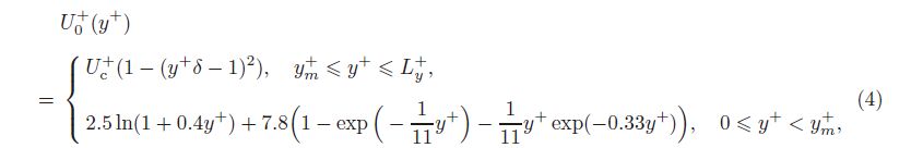
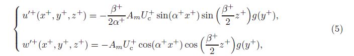
For the lifted low-speed streak initially free of the initial streamwise vortex, we adopt the streamwise velocity distribution proposed by Schoppa and Hussain^[20] to represent the initial straight streak in the streamwise direction:

where Δu⁺ is the streak velocity defect, Δu⁺ = 11.2, the superscript ⁺ denotes the wall unit, β⁺ is the spanwise wave number, determining the spanwise spacing between two spanwise aligned low-speed streaks, and β⁺ = π/50. To make sure that the turbulent active region is located near y⁺ = 30, a normalized function defined by is employed, where σ⁺ = 5.5 × 10^-4.

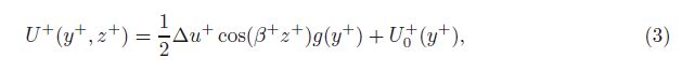
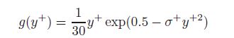
For the flow velocity distribution (U₀⁺ (y⁺) in Eq. (3)), the one-sided turbulent flow^{[20, 25]} is constructed and expressed as follows:

where U_c⁺ is the maximum mean velocity at the centerline of the channel. It is defined by U_c⁺ = 1.0/u_τ, where u_τ is the friction velocity acquired by Dean’s empirical correlation^[26], In the above equation, h is the half height of the channel, h=1, and δ is the viscous length unit defined by δ = υ/u_τ . The velocity when y_m⁺ ≤ y⁺ ≤ L_y⁺ represents the laminar flow, whereas the velocity when 0 ≤ y⁺ < y_m⁺ represents the turbulent flow.

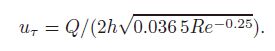
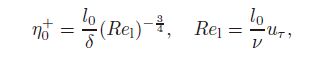
To establish two spanwise aligned straight streaks with the mean spanwise spacing of 100 in wall unit^{[1, 5, 25, 27, 28, 29]} on the lower wall of the channel, the spanwise length (L_z⁺ ) of the channel is taken to be 200 in wall units. The streamwise length (L_x⁺ ) of the channel is taken to be 300 in wall units, which statistically represents the streamwise length scale of a typical vortex^[30]. The normal height (L_y⁺ ) is taken as L_y⁺ = 2h/δ = 328 based on the viscous length δ and the half height of the channel h. With 64 × 129 × 64 computational grid points in (x, y, z ), Δx⁺ = 4.7 (about 1.31η₀⁺, where η₀⁺ is the Kolmogorov length scale obtained by

in which l₀ is near wall integral scale, and l₀ = h), Δy⁺ ranges from 0.05 (about 0.014η₀⁺) at the wall to 4 (about 1.12η₀⁺) at the center of the channel, and Δz⁺ = 3.125 (about 0.87η₀⁺), which are comparable to the sizes used by Kim et al.^[31] and Jiménez and Moin^[25] with similar Reynolds numbers. They are sufficient to resolve the essential turbulent scales^[32].

To excite the instability of the low-speed streaks, the initial perturbations are proposed to allow the streak instability developing in the SV mode, i.e.,

where u′⁺ and w′⁺ denote the streamwise and spanwise perturbation velocities in wall unit, respectively. α⁺ is the streamwise wave number of the perturbations, which determines the oscillation frequency of the low-speed streaks in the streamwise direction, and α⁺ = 2π/300. β⁺ is the same as that described in Eq. (3) to ensure that the perturbations can match the lowspeed streaks with the same spanwise position. A_m is the streak transient growth (STG)^[20] perturbation amplitude, and its critical value to keep the SV low-speed streaks sustaining is A_m = 0.07, which is obtained by a few simulations with different perturbation amplitudes. It is worth noting that the critical value of A_m to keep the SS low-speed streaks sustaining is less than 0.02, which is much less than that of the SV low-speed streaks (A_m = 0.07). This means that the SV low-speed streaks are less sensitive to the initial perturbation amplitude than the SS low-speed streaks. This further confirms that the low-speed streaks with the sinuous mode are more unstable than those of the varicose mode^{[6, 7, 8, 9, 10]}. Besides, the perturbations expressed by Eq. (5) not only ensure the divergence-free condition of the flow field, but also trigger the instability pattern of the SV mode between the low-speed streaks (see Fig. 1).

The mean streamwise velocity profiles and the Reynolds shear stress profiles in wall unit in the present channel flow, U⁺(y⁺) and u⁺v⁺(y⁺), ranged from t⁺ = 2 500 to t⁺ = 6 000, are compared with the experimental results of Wei and Willmarth^[33] and Niederschulte et al.^[34] in the fully developed channel flow with approximately the same Reynolds numbers (see Figs. 2(a) and 2(b)). The good agreement of the statistical properties at the late stage in this local region with those in the fully developed turbulence is clearly visible, indicating that the fully developed turbulence originated from the low-speed streaks with the SV mode in the present channel can be formed and can represent the physical realization of the turbulence. The dynamics of the low-speed streaks and the streamwise vortices in phenomenological view will be presented in the next section.

3 Results and discussion 3.1 General dynamical process of evolution of low-speed streaks

The evolution of the low-speed streaks (characterized by the instantaneous streamwise velocity u⁺) and the streamwise vortices (characterized by the streamwise vorticity) is shown in Fig. 3. A typical behavior at the early stage is the occurrence of the streamwise vortex sheets in the overlapping pattern with the alternating signs located between two SV low-speed streaks near the wall (see Fig. 3(a)). After a short time, each of the streamwise vortex sheets inclines in the z-direction, and the oppositely signed zigzag vortex sheets are formed in pairs along the x-direction (see Fig. 3(b)). At t⁺ = 100 in Fig. 3(c), the zigzag streamwise vortex sheets shown in Fig. 3(b) soon stretch into the tilted streamwise vortex tubes attached to the flanks of each streak, thus lifting the low-speed streaks. At the same time, new V -like streamwise vortices are formed at the crown of the low-speed streaks, leading to the downward motion of the streaks. When the streamwise vortices are further enhanced, the SV low-speed streaks continue intensifying till breakdown occurs at t⁺ = 217 (see Fig. 3(d)). The breakdown of the low-speed streaks can lead to the viscous decay of the low-speed streaks (see Fig. 3(e)), and the new zigzag streamwise vortices between the two low-speed streaks near the wall can be regenerated and accompanied by the breakdown of the low-speed streaks (see Figs. 3(d) and 3(e)). It is noted that the new generated zigzag streamwise vortices at t⁺ = 272 (see Fig. 3(e)) are nearly the same as those at t⁺ = 45 (see Fig. 3(b)). Therefore, the next sustaining evolution cycle of the SV low-speed streaks including intensification (see Fig. 3(f)), breakdown (see Fig. 3(g)), and decay (see Fig. 3(h)) can be triggered, whose evolution process is similar to that of the first sustaining cycle. However, the streamwise vortices in the second sustaining cycle are much stronger (see Fig. 3(f)), and their shapes are more chaotic (see Fig. 3(g)) than those of the first sustaining cycle (see Figs. 3(c) and 3(d)). Most significantly, the streamwise vortices at t⁺ =787 decay from the bottom to the top (see Fig. 3(h)), and only the V -like streamwise vortices are kept, which are quite different from the decay of the first sustaining cycle (see Fig. 3(e)). As time goes on, the V -like streamwise vortices are re-enhanced on the top of the decayed streaks (see Figs. 3(i), 3(j), and 3(k), inducing the weak spanwise-aligned low-speed streaks into the pattern of the SS mode with a half shift of the spanwise wavelength phase (see Fig. 3(k)). With the enhancement of the streamwise vortices, the SS low-speed streaks are intensified (see Fig. 3(k)), and subsequently break down (see Fig. 3(l)), whose evolution is the same as that in Ref. ^[15]. The above scenario indicates two main features. One is that the development of the low-speed streaks strongly depends on the strength of the streamwise vortices, and vice versa. The unstable SV low-speed streaks can lead to the formation and enhancement of the tilted and V -like streamwise vortices, which in turn can intensify the SV low-speed streaks. The other is that the SV low-speed streaks cannot be kept permanently, but transform into the SS low-speed streaks, which implies the dominant role of the SS low-speed streak instability in the near-wall turbulence^{[11, 14]}. These features will be discussed in depth in the next sections.

3.2 General dynamical process of evolution of low-speed streaks

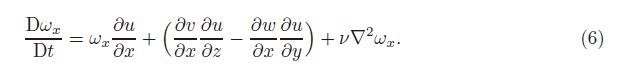
The dynamics of the streamwise vortices can be obtained by considering the transport evolution equation for the streamwise vorticity:

The three terms on the right-side of Eq. (6) represent the variations of the streamwise vorticity due to stretching, tilting, and viscous diffusion, respectively, and the root mean square profiles of the three terms at four selected time during the first sustaining cycle are shown in Fig. 4. At t⁺ = 9 (see Fig. 4(a)), the tilting term dominates the evolution of the streamwise vorticity, but the stretching term is neglected. Therefore, the streamwise vortex sheets in Fig. 3(a) are mainly contributed by the tilting term. At this instant, the viscous diffusion mainly concentrates on the bottom of the channel. At t⁺ = 100 (see Fig. 4(b)), the stretching term increases rapidly, resulting in the formation of the streamwise vortex tube (see Fig. 3(c)). At this time, the tilting term and the viscous diffusion term increase away from the wall. When the low-speed streaks break down, all terms have two peaks (see Fig. 4(c)): the first peak is near y⁺ = 15, and the second peak is near y⁺ = 55. The former corresponds to the zigzag vortices near the wall (see Fig. 3(d)), the latter corresponds to the streamwise vortices and V -like streamwise vortices (see Fig. 3(d)). When the low-speed streaks decay, the second peak of the three terms in Fig. 4(c) disappears, but the first peak remains (see Fig. 4(d)), resulting in the retained zigzag streamwise vortices (see Fig. 3(e)).

Schoppa and Hussain have shown that single sinuous low-speed streaks can lead to the formation of the streamwise vortex sheets by the shearing mechanism^[20] mainly contributed by the vorticity tilting, and the vortex sheets soon enhance into the vortex tubes by stretching of +$\frac{\partial u}{\partial x}$ ^[20]. From Fig. 4, it can be concluded that this mechanism is still suitable for the case of SV low-speed streaks. Since the viscous diffusion increases with the vorticity tilting and stretching, the competing of them can lead to the quasi-periodic development of the low-speed streaks and streamwise vortices. In this subsection, we discuss the intensification of the streamwise vortices by the shearing and stretching mechanisms and the relationship between the streamwise vortices and the low-speed streaks. The breakdown and decay of the streamwise vortices and the lowspeed streaks will be presented in the next subsection.

Figures 5 and 6 illustrate the formation of the streamwise vortex sheets generated by the SV low-speed streaks. At the initial time (t⁺ = 0) (see Fig. 5(a)), due to the no slip condition at the wall (w⁺ = 0 at y⁺ = 0) and the elliptical spanwise velocity region (near y⁺ = 30) triggered by the initial spanwise perturbation with Eq. (5), the flattened streamwise vorticity dominated by the spanwise velocity gradient ($\frac{\partial {{w}^{+}}}{\partial {{y}^{+}}}$) can be formed near the wall. After a short time (see Fig. 5(b)), the spanwise velocity regions shear-deform into the tilted shape along the streamwise direction due to the increase in the streamwise velocity with the distance from the wall. With +w⁺ over the top of -w⁺ near x⁺ = 150 (see Fig. 6), $\frac{\partial {{w}^{+}}}{\partial {{y}^{+}}}$ is formed not only near the wall but also between +w⁺ and -w⁺. This gives birth to the overlapped and tilted streamwise vortex sheets (see Fig. 3(a)). Note that the streamwise vortex sheets generated by the SV low-speed streaks are located between two streaks (see Fig. 3(a) and Fig. 6), whereas the vortex sheets generated by the SS low-speed streaks attach on each streak (see Figs. 8(c) and 8(d) in Ref. ^[15]). Such a difference is caused by the positions of the initial spanwise velocities induced by different initial perturbation equations. For the SS low-speed streaks, the initial spanwise velocity regions attach on each sinuous streak (see Fig. 8(b) in Ref. ^[15]). For the SV low-speed streaks, the initial spanwise velocity regions are located between two low-speed streaks (see Fig. 6). Therefore, the shearing motion of the initial spanwise velocity region does not happen on each of the SS low-speed streaks, but happens between two streaks of the SV low-speed streaks, leading to different positions of the streamwise vortex for the SS low-speed streaks and the SV low-speed streaks. Although the positions of the vortex sheets generated by the SS low-speed streaks and the SV low-speed streaks are quite different, similar vortical structures indicate that the formation mechanisms of the streamwise vortex sheets for both cases are caused by the shearing of the initial spanwise velocity regions.

Once the overlapping regions between two streamwise vortex sheets form (see Fig. 3(a)), each of the sheets inclines in the spanwise direction due to the mutual induction effect^{[15, 35]}, resulting in the zigzag streamwise vortices (see Fig. 3(b)). Figure 7 gives the streamwise vortices colored by the local values of the spanwise velocity (w⁺) to illustrate the spanwise motion of the streamwise vortices. Here, the streamwise vortices are marked by SV_I+, SV_I-, SV_II+, and SV_II-, where the subscripts I and II correspond to the streamwise vortices near z⁺ = 100 and z⁺ = 200 (or 0), respectively, and the subscripts + and - indicate different rotating directions of the streamwise vortices. It can be seen that large spanwise velocities concentrate on the overlapping parts of the streamwise vortices, where the alternative spanwise velocities have a half shift of the streamwise wavelength phase from each other. This can be explained by the mutual induction referred in Ref. ^[15], i.e., the mutual induction effect between the upstream tail of SV_I+ and the downstream head of SV_I- based on the Biot-Savart law can lead to the positive spanwise motion in the overlapping region (x⁺ = 100). Similarly, the mutual induction effect between the downstream head of SV_I+ and the upstream tail of SV_I- can result in the negative spanwise motion in the overlapping region (x⁺ = 250). Therefore, for the single streamwise vortex, e.g., SV_I+, different spanwise motion for the head and the tail leads to the spanwise inclination of the streamwise vortex. By the symmetry, the mutual induction effect between SVII⁺ and SV_II- can also be triggered, leading to the inclination of the streamwise vortices but the inclined direction is opposite to SV_I+ and SV_I-. Because of this reason, two pairs of zigzag streamwise vortex sheets with opposite spanwise inclinations are formed, and the low-speed streaks under this circumstance become unstable (see Fig. 3(b)).

Once the SV low-speed streaks become unstable, the streamwise vortex sheets can be stretched into the streamwise vortex tubes by increasing +$\frac{\partial u}{\partial x}$. The relationship between $\frac{\partial u}{\partial x}$ and the streamwise vortices is presented in Fig. 8. From the figure, we can see that the crest of the low-speed streak is lifted and rolled up. This increases the streamwise velocity difference along the x-direction, hence leading to larger $\frac{\partial u}{\partial x}$. Consequently, large +$\frac{\partial u}{\partial x}$ develops the downstream of the lifted streak, leading to the generation and enhancement of the tilted and V -like streamwise vortices^[20]. On the other hand, the tilted streamwise vortices and V -like streamwise vortices can in turn increase the bending amplitude of the low-speed streak. As a result, the positive feedback between the low-speed streaks and the streamwise vortices occurs till the low-speed streaks break down.

3.3 Breakdown of SV low-speed streaks

It has been shown in Fig. 3(d) that the oppositely signed zigzag streamwise vortices can be generated in pairs along the x-direction accompanied by the first breakdown of the SV low-speed streaks, and hence giving birth to the second sustaining cycle. To examine the generation of the zigzag streamwise vortices between two SV low-speed streaks, Fig. 9 gives the low-speed streaks drawn by $\frac{\partial {{u}^{+}}}{\partial {{x}^{+}}}$ and the normal velocity (v⁺) at t⁺ = 217. One can see that +v⁺ and -v⁺ near z⁺ = 100 are alternatively arranged both in the streamwise direction and the spanwise direction, respectively. Since +v⁺ induces upward motion of the low-speed fluid from the vicinity of the wall, weak sinuous low-speed streaks can be formed between two SV low-speed streaks near the wall. Consequently, a sizable sinuous region of +$\frac{\partial {{u}^{+}}}{\partial {{x}^{+}}}$ is formed at the downstream side of +v⁺ on account of the increasing streamwise velocity difference along the x-direction, leading to the generation of zigzag streamwise vortices (see Fig. 3(d)).

However, when the second breakdown of the SV low-speed streaks happens, the regeneration of the SV low-speed streaks is terminated. From Fig. 10, one can see the weak and chaotic distribution of the normal velocity between the two SV low-speed streaks near the wall (z⁺ = 100), indicating that the sinuous $\frac{\partial u}{\partial x}$ and the zigzag streamwise vortices under this circumstance cannot be generated. Note that the strength of the streamwise vortices at t⁺ = 588 (see Fig. 3(g)) is much stronger than that at t⁺ = 217 (see Fig. 3(d)), but the normal velocity near the wall at t⁺ = 588 (see Fig. 10) is relatively weaker than that at t⁺ = 217 (see Fig. 9). This is because that the streamwise vortices generated by the second breakdown of the SV low-speed streaks are located far from the wall and can barely induce the normal velocity between the two streaks near the wall. For this reason, zigzag streamwise vortices are inhibited, and the regeneration of the SV low-speed streaks is terminated.

Another difference between the first breakdown and the second breakdown of the SV lowspeed streaks is that each low-speed streak can induce a pair of new V -like streamwise vortices besides the primary one at the second breakdown. Here, we call the new generated one as the secondary V -like streamwise vortices. The formation of the secondary V -like streamwise vortices is illustrated in Fig. 11. One can see that the secondary V -like streamwise vortices resided on the surface of the broken isolated low-speed region coincide with the peak of +$\frac{\partial {{u}^{+}}}{\partial {{x}^{+}}}$. Since the tilted streamwise vortices are fully stretched and their tips (x⁺ ∈ [100,140] and y⁺ ∈ [100,120] in Fig. 11) have reached the upstream tail of the broken isolated low-speed region, the upstream tail of the broken isolated low-speed region can be lifted by the induction of the tips of the tilted streamwise vortices. As mentioned above, the lifted motion of the low-speed streak is in favor of the +$\frac{\partial {{u}^{+}}}{\partial {{x}^{+}}}$ downstream. Therefore, the secondary V -like streamwise vortices are formed at the downstream side of the +v⁺, corresponding to the region of large +$\frac{\partial {{u}^{+}}}{\partial {{x}^{+}}}$ (see Fig. 11). It is noteworthy that the lifted upstream tail of the broken isolated low-speed region is caused by the stretching motion of the tilted streamwise vortices. At t⁺ = 217 (see Fig. 3(d)), the strength of the tilted streamwise vortices is too weak to lift the tail of the broken isolated low-speed region, and the secondary V -like streamwise vortices under this circumstance cannot be formed.

3.4 Transformation from SV to SS

Before discussing the transformation from SV low-speed streaks to SS low-speed streaks, one should clarify how these streamwise vortices develop after the second breakdown of lowspeed streaks. Figure 12 gives several streamwise vortices whose iso-surfaces are colored by the distribution of +$\frac{\partial {{u}^{+}}}{\partial {{x}^{+}}}$. It can be found that large +$\frac{\partial {{u}^{+}}}{\partial {{x}^{+}}}$ concentrates at the secondary V -like streamwise vortices, implying that the tilted streamwise vortices and the first V -like streamwise vortices decay rapidly but the secondary V -like streamwise vortices remain the same as time goes on (see Fig. 3(h)).

Once the tilted streamwise vortices and the first V -like streamwise vortices disappear, the decayed low-speed streaks can only be affected by the remaining secondary V -like streamwise vortices. Figure 13 shows the evolution of the remaining secondary V -like streamwise vortices and the left streak profile. From t⁺ = 787 (see Fig. 13(a)) to t⁺ = 869 (see Fig. 13(b)), the decayed low-speed streak is gradually separated and divided into two parts by the sweep motion of the V -like streamwise vortices. Similar separated motion can take place on the right varicose low-speed streak with a half shift of the streamwise wavelength phase.

Figure 14 gives the transformation of the low-speed streaks from the SV mode to the SS mode. One can see from t⁺ = 869 (see Fig. 14(a)) to t⁺ = 1 032 (see Fig. 14(b)) that the right part of the original left varicose streak (see Region A in Fig. 14(a)) gradually combines with the left part of the original right varicose streak (see Region B in Fig. 14(a)), ultimately leading to the formation of the new sinuous streak at z⁺ = 100 (see Fig. 14(b)). Simultaneously, Region C gradually combines with Region D, giving birth to another new sinuous streak at z⁺ = 0 (z⁺ = 200), which has an opposite spanwise oscillation. As a result, new SS lowspeed streaks are formed, and their positions are shifted in the spanwise direction with a half wavelength phase compared with those of the original SV low-speed streaks. The positive feedback between the SS low-speed streaks and the streamwise vortices finally lead to the development and breakdown of the streaks (see Figs. 3(k) and 3(l)), which has been described in Ref. ^[15].

4 Conclusions

Based on the Fourier-Chebyshev spectral method, a DNS is used to investigate the development of two spanwise-aligned subharmonic varicose (SV) low-speed streaks in a small periodic channel flow. The results show that the SV low-speed streaks are self-sustained at the early stage but finally transformed into SS low-speed streaks, which play a dominating role for the streak instability in both transitional and developed turbulent boundary layer flows.

Initially, the streamwise vortex sheets are formed between two SV low-speed streaks near the wall due to the shearing mechanism. Since the oppositely signed streamwise vortex sheets overlap in the streamwise direction with each other, the mutual induction between the vortices happens, leading to the spanwise inclination of the streamwise vortex sheets. Then, the lowspeed streaks under this circumstance become unstable, directly leading to the formation of tilted streamwise vortex tubes and V -like streamwise vortex tubes by increasing $\frac{\partial u}{\partial x}$. The tilted streamwise vortices and V -like streamwise vortices can increase the bending amplitude of the low-speed streaks, while the three-dimensional bending low-speed streak can increase the +$\frac{\partial u}{\partial x}$ downstream that in turn enhances the strength of the streamwise vortices. Thus, positive feedback between the streamwise vortices and the streaks can be triggered till the SV low-speed streaks break down. Once breakdown occurs, new zigzag streamwise vortices and sinuous +$\frac{\partial u}{\partial x}$ can be formed since the oppositely signed normal velocities are alternatively arranged in both the streamwise direction and the spanwise direction. This can lead to the next sustaining cycle of the SV low-speed streaks whose behavior is nearly the same as that of the first sustaining cycle.

However, the regeneration of the SV low-speed streaks never happens after the second breakdown since the sinuous +$\frac{\partial u}{\partial x}$ and the zigzag streamwise vortices cannot be formed. Meanwhile, the new secondary V -like streamwise vortices can be generated near the location of the large value of +$\frac{\partial u}{\partial x}$ in the broken isolated low-speed region. As time goes on, all of the vortices but the secondary V -like streamwise vortices decay, and the decayed streaks can only be affected by the remaining secondary V -like streamwise vortices. Each decayed low-speed streak is divided into two parts by the sweep motion of the secondary V -like streamwise vortices, and gradually combines with another separated streak, finally leading to the formation of the SS low-speed streaks.