1 Introduction

Turbulence is the basic flow state in nature. However, it has still not been well understood. The prediction of the laminar-turbulent transition is very important to the design and man- ufacture of vehicles, ships, and aircrafts. According to the classical stability theory, at low turbulence level, unstable Tollmien-Schlichting (T-S) waves are first excited in the boundary layers, and then grow linearly until a breakdown occurs. Receptivity establishes the initial con- ditions of the amplitude, the frequency, the wave number, and the phase for the breakdown of the laminar flow^[1]. Current understanding shows that the boundary-layer receptivity to acous- tic and vortical disturbances occurs in the regions where there is a rapid streamwise variation in the mean-flow such as at the leading edge of the flat-plate^[2] and at the wall roughness^[3].

Alzin and Polyakov^[4] demonstrated the local receptivity mechanism by experiments, and measured a linear increase in the receptivity with the acoustic forcing and roughness height. Goldstein^[3] and Ruban^[5] independently showed that the local short-scale mean flow distortion due to a roughness element was capable to excite the short-wavelength T-S waves with long- wavelength acoustic waves, i.e., the wavelength conversion mechanism.

For the vortical receptivity, Rogler and Reshotko^[6] modeled the free-stream disturbances as an array of counter-rotating convected vortices to analyze the boundary-layer response. Zavol’skii et al.^[7] noted that the most effective T-S wave excitation occurred at the resonance condition

where α_wall is the wave number of the roughness element. Crouch^[8] adopted the convected vortices model used by Rogler and Reshotko^[6] to study the local receptivity at the distributed roughness. Based on the multi-scale asymptotic techniques, Duck et al.^[9] found that any roughness on the wall might cause T-S wave generation in the boundary layer under vortical disturbances. Dietz^{[10, 11, 12]} carried out the experimental verification for the local receptivity to vortical disturbances. Promoted by these experiments, Wu^[13] presented a second-order asymptotic theory to study the local receptivity to vortical disturbances, and the obtained results agreed well with Dietz’s measurements. Zhang and Zhou^[14] confirmed the range of validity of the linear receptivity formula by using the direct numerical simulation (DNS).

Many studies on vortical receptivity involve single-frequency vortical disturbances^{[12, 13, 14]}, whereas the studies on the receptivity to broadband free-stream turbulence (FST) are relatively less. In this paper, the boundary-layer receptivity under the interaction of FST and localized wall roughness is studied by the DNS and fast Fourier transformation. The obtained results agree well with Dietz’s experiments^{[11, 12]} and Zhang and Zhou’s numerical data^[14].

2 Governing equations and numerical methods 2.1 Governing equations

The dimensionless Navier-Stokes equations are

where V = U +V ′, and U is the Blasius solution. V ′ = (u, v)^T is the perturbation velocity. p is the pressure. The Reynolds number is defined by Re = (U_∞δ^*)/ν, where δ^* is the boundary- layer displacement thickness. U_∞ is the free-stream velocity. ν is the kinematic viscosity.

2.2 Numerical methods

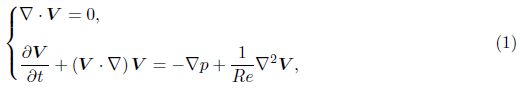
High-order finite difference schemes are introduced to discretize the governing equations (1). For the time integration, a modified fourth-order Runge-Kutta scheme is employed^[15]. A spectral method is used for the x-direction discretization, and non-uniform compact finite difference schemes are used for the y-direction discretization. The detail is presented in Ref. ^[16].

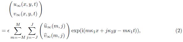
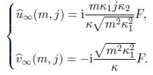
2.3 Free-stream turbulence model

The mathematical model^[17] is introduced to generate the FST, which is represented by

where Here, $F=\sqrt{\frac{2E(\kappa ){{\kappa }_{1}}{{\kappa }_{2}}}{4\pi {{\kappa }^{2}}}}{{e}^{i\theta }}, i=\sqrt{-1}$, $\epsilon$ denotes the amplitude, κ₁ and κ₂ are the fundamental wave numbers in the x-direction and y-direction, respectively, and ${{\hat{u}}_{\infty }}$ and ${{\hat{u}}_{\infty }}$ depend on the one-dimensional energy spectrum E(κ) and the random angle θ. For a real reflection of the random nature of the actual turbulence, the frequencies of the proposed FST model can be arbitrarily selected. In this study, the frequencies of the FST are selected to cover the frequency range of the neutral stability curves for the excitations of the instability T-S waves, which are important in the laminar-turbulent transition.

2.4 Computational domain

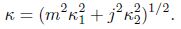
The computational domain is the shadow area in Fig. 1. The length of the domain is X = 2.0 × 2π/κ₁ so that the generated waves cannot reach the exit and the height of the domain Y = 14.39 is five times of the boundary-layer thickness:

The roughness element is placed at the location X/16 from the entrance. 1 024 × 200 grids are arranged in the x-direction and the y-direction, respectively. The grids in the x-direction are uniform. The refined grids are utilized near the wall in the y-direction, which are given by

where

2.5 Boundary conditions

According to Ref. ^[17], the perturbation velocity of the imposed FST at the upper boundary is

The boundary conditions at the wall are The localized roughness elements are added on the wall. The rectangle element is the sine element is and the triangle element is where h is the roughness height, and U′(0) is the first derivative of the base flow on the wall. x_w ∈ [x₁, x₂], where x₁ is the start of the roughness elements, and x₂ is the end. Therefore, the roughness width L = x₂ - x₁. The zero pressure gradient condition is set on the wall. The periodical boundary conditions are applied in the streamwise direction. The initial conditions are

3 Numerical results and discussion 3.1 Boundary-layer receptivity under interaction of FST and localized wall rough-ness

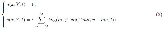
In this section, we focus on the boundary-layer receptivity to the FST interacting with the localized wall roughness. The amplitude of the FST is set to 0.001, and a rectangle hump of the height 0.05 and the width X/128 is added to the surface of the plate. Hereafter, ω and α are the frequency and the streamwise wave number, respectively.

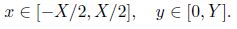
As shown in Fig. 2, a group of generated perturbation wave packets are observed at the Reynolds number 800, which is determined by a subtraction of the result computed above a smooth plate from a similar numerical result with the localized wall roughness, where the arrows in the figures point at the roughness location. Figure 2(a) plots the spatial evolu- tion of the perturbation wave packets in the boundary layer at t = 1 050, and its amplitude increases in the streamwise direction. Figure 2(b) gives the temporal evolution of the wave packet at a fixed point x = -150 in the boundary layer, whose amplitude is constant over time. According to the evolution of the wave packets, the positions of the peaks and valleys are tracked over time to calculate the propagation speed by taking the average. The propagation speed of the wave packets is 0.370.

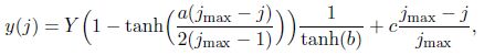
Then, a group of perturbation waves are separated from the wave packets in Fig. 2(a) by the fast Fourier transformation. The spatial evolutions of these stability, neutral, and instability waves are plotted in Figs. 3(a), 3(b), and 3(c), respectively. According to the spatial evolutions, the frequencies, the wavelengths, and the growth rates (or decaying rates) of the isolated waves can be estimated by the averages of the periods, the distances between the peaks/valleys and the neighbor peaks/valleys, and the amplitude ratios of the peaks/valleys to their neighbor peaks/valleys.

The excited wave packets at the Reynolds numbers 520, 800, and 1 000 are treated in the same way, and the results are presented in Tables 1, 2, and 3. As shown in Tables 1, 2, and 3, the generated perturbation waves in the boundary layer have different dispersion relations from those of the imposed FST. They share the same frequencies, but the gener- ated waves have shorter wavelengths (or larger wave numbers), which confirms the wavelength conversion mechanism for the receptivity^{[9, 12, 13]}. Moreover, the dispersion relations of the excited perturbation waves are identical with the theoretical solutions of the T-S waves ob- tained from the Orr-Sommerfeld (O-S) equation, and the errors between them are less than 10^-4. In addition, at the critical Reynolds number 520, only one neutral wave is excited (see Table 1). At the Reynolds number 800, the frequencies of the excited neutral waves are ω = 0.066 20 and ω = 0.136 24, which are exactly on the lower and upper branches of the neutral stability curve, and the frequencies of the excited instability waves are within these two branches (see Table 2). Similarly, at the Reynolds number 1 000, the frequencies of the excited instability waves are ω = 0.054 48 and ω = 0.130 00, which are exactly on the lower and upper branches of the neutral stability curve, and the frequencies of the excited instability waves are within these two branches (see Table 3). These results agree with the theoretical solutions of the neutral stability curve. Furthermore, the parameters of the free-stream turbulence model of the upper and lower branches in Tables 1, 2, and 3 are arbitrarily selected. In theory, an infinite number of small perturbation waves can be chosen. For calculational feasibility, we only consider the free-stream turbulence model consisting of a finite number of small perturbation waves, interacting with the wall roughness to generate T-S waves in the boundary layer. These indirectly validate the randomness of the free-stream turbulence, and also illustrate that the proposed free-stream turbulence model has the features of natural turbulence.

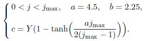
The neutral wave when α = (0.124 00, 0.000 00) and ω = 0.311 25 is selected from Table 1 as an example for the discussion, and Fig. 4 gives a rigorous comparison between the amplitude and phase of the neutral wave and the solutions of the O-S equation. The results agree perfectly with each other.

The frequencies, wave numbers, growth rates (or decaying rates), amplitudes, and phases of the generated perturbation waves do match the theoretical solutions of T-S waves obtained from the O-S equation. It demonstrates that the T-S wave packets superposed by a group of stability, neutral, and instability T-S waves are excited by the FST interacting with the localized wall roughness, thus confirming that boundary-layer receptivity exists.

Furthermore, the computed propagation speed of the T-S wave packets in the boundary layer is 0.391, 0.370, and 0.350 with the Reynolds numbers of 520, 800, and 1 000, respectively, which is approximately one-third of the free-stream velocity, closely matching the propagation speeds of the T-S wave packets measured by Dietz^[11]. The phase speed of the neutral T-S waves in Table 1 is 0.398, and the phase speeds of the most unstable T-S wave in Tables 2 and 3 are 0.367 and 0.355, respectively. It indicates that the propagation speeds of the T-S wave packets are largely determined by the phase speeds of the most unstable T-S waves.

3.2 Receptivity response to forcing amplitude, roughness height and width

Dietz’s experiment data^[12], Wu’s theoretical study^[13], and Zhang and Zhou’s numerical results^[14] have verified that for single-frequency vortical disturbances interacting with localized wall roughness, the receptivity response is linear within a specific range. The linear receptivity formula is

where u_TS is the amplitude of the generated T-S wave, u_FS is the amplitude of the free-stream disturbance, and F(α_TS -α_FS) is the spatial transform of the roughness geometry at the wave number difference between the T-S wave number α_TS and the wave number of free-stream disturbance α_FS. The efficiency function Λ(ω, Re) is independent of the roughness geometry.

The Reynolds number is accordingly set to the same as that in Dietz’s experiment^[12]. In Figs. 5 and 6, |u₀| is the amplitude of the excited T-S wave in the boundary layer when

and |u_max| is the amplitude of the T-S wave excited by a rectangle hump of width π/(α_TS-α_FS). Figure 5(a) gives the variations of the excited T-S wave amplitude with the amplitude of the imposed FST, where the amplitude of free-stream turbulence u_FS corresponds to the amplitude at the edge of the boundary layer. The boundary-layer receptivity is found to be linear for the forcing amplitude up to 1% of the free-stream velocity. Figure 5(b) shows that for the non- dimensional height h^*/δ_r less than 0.2, the receptivity responses of the generated T-S waves with different frequencies are all linear, where h^* is the dimensional height, and δ_r = (νx/U_∞)^1/2 is the boundary-layer reference height. These agree well with Dietz’s experiment^[12] and Zhang and Zhou’s numerical results^[14] for vortical receptivity, and are also similar to those found for acoustic receptivity by Bodonyi^[18], Saric et al.^[19], and Zhou et al.^[20].

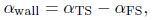
The spatial Fourier transformation of the roughness geometry evaluated at (α_TS - α_FS) for a single rectangle hump is given by

Figure 6 gives the variations of the T-S wave amplitude with the roughness width, where L is normalized by the resonant wave length 2π/(α_TS - α_FS). The computed results are found to agree with the function sin(L(α_TS -α_FS)/2), which is a factor of Eq. (8). When the roughness width is equal to π/(α_TS -α_FS), the maximum amplitude of the T-S wave is excited. Figure 7 shows that the receptivity response is almost linear with the spatial Fourier transformation of the roughness geometry. These results reach the same conclusions with Dietz’s experiments^[12] and Zhang and Zhou’s calculations^[14].

In conclusion, Eq. (7) is demonstrated to be also valid for the multi-frequency T-S waves generated by the FST interacting with the localized wall roughness when the forcing amplitude is less than 1% of the free-stream velocity and the non-dimensional height h^*/δ_r is less than 0.2.

3.3 Receptivity response to different roughness geometries

The receptivity response to different roughness geometries is studied under the FST. Six different roughness geometries (rectangle, sine, and triangle humps/gaps) are solely added on the wall with the same cross-section area. The heights of the rectangle, sine, and triangle hump/gap are

respectively, and the widths are 6.33.

As shown in Table 4, the dispersion relations of the T-S waves excited by the roughness elements of different geometries are almost identical, which also agree well with the solutions of the O-S equation. It indicates that the dispersion relations of the generated T-S waves cannot be changed by varying the geometry of the roughness elements. However, the variations of the roughness geometries are able to change the phases and amplitudes of the generated T-S waves. As seen in Fig. 8, the T-S waves with opposite phases are generated by a sine hump and a sine gap, respectively, and the amplitudes of the T-S waves generated by a sine hump are larger than those generated by a sine gap. Similar conclusions are found with the rectangle and triangle roughness elements.

4 Conclusions

The boundary-layer receptivity under the interaction of free-stream turbulence and localized wall roughness has been studied by the DNS and fast Fourier transform. The free-stream turbulence model is set up to reflect the nature of real turbulence which is random and consists of multi-frequency and multi-scale fluctuations. As a result, T-S wave packets are observed, which are superposed by a group of stability, neutral, and instability T-S waves excited in the boundary layer. The propagation speeds of the T-S wave packets, which are approximately one-third of the free-stream velocity, are found to be largely determined by the phase speeds of most unstable T-S waves. Rather than the excitation of a single T-S wave^{[12, 13, 14]}, the boundary- layer receptivity to the FST in the present study is more universal. The linear receptivity formula is demonstrated to be valid for the multi-frequency T-S waves generated by the free- stream turbulence when the forcing amplitude is up to 1% of the free-stream velocity and the non-dimensional height h^*/δ_r is less than 0.2. These conclusions are similar to those found by Dietz^{[11, 12]} and Zhang and Zhou^[14]. Additionally, the effects of the roughness geometries on the receptivity are also studied. It is found that the dispersion relations of the generated T-S waves cannot be changed by varying the geometry of the roughness elements with the same cross-section area and width, whereas the phases and amplitudes of the generated T-S waves are changed.