1 Introduction

Kidneys are naturally installed filtration plants in the body of several living beings. The glomerular filtration rate is in the range from 150 liters to 170 liters per day, of which only 1.0 liter to 1.5 liters come out as urine^[1]. Whenever kidneys stop filtering properly, the artificial kidneys (dialyzer) will be capable of postponing death from the irreversible kidney failure within a few years. Nephron is the basic unit of kidneys, having small tubules named as renal tubules where the filtered liquid is absorbed through small pores. Normally, the size of the pores on the surface of a tubule remains to be uniform. However, due to the growth of microorganisms, they sometimes become narrow or get blocked, i.e, biofouling. It is observed and graphically shown by Azar et al.^[2] that the efficiency of the dialyzer goes down due to the adsorption of the protein on the surface of the membrane that decreases the diffusive and convective transport of blood during the dialysis process. The velocity and pressure fields in these situations differ from simple Poiseuille flow since the fluid in contact with the wall has a normal velocity component. These velocity components and pressure drops have been calculated by Berman^[3]. He worked out this problem with the inertia term by use of the similarity method. Later, Sellars^[4], Yuan^[5], and Terrill^{[6, 7]} further studied and extended the work of Berman^[3].

Wesson and Lawrence^[8] and Burgen^[9] theoretically discussed the renal model by assuming a constant rate of absorption. Due to the reason that the biofouling radial velocity may not remain to be constant or be known in advance, Macey^[10] relaxed the condition of constant absorp- tion, and included the possibility of the absorption rate that varied linearly with the distance. Kelman^[11] demonstrated that the bulk flow in the proximal tubule decayed exponentially. Mo- tivated by the work of Kelman, Macey^[12] considered a more general boundary condition. He obtained the explicit solutions for the axially symmetric creeping flow in an infinite permeable cylinder by use of exponential absorption. Kozinski et al.^[13] modified Macey’s work in tubes and extended it for porous slits. Marshll and Trowbridge^[14] and Palatt et al.^[15] used the phys- ical conditions existing in the permeable tube instead of prescribing the flux/radial velocity, and studied fractional absorption and leakage flux. Radhakrishnamacharya et al.^[16] studied the creeping flow through the renal tubule by the hydrodynamic aspect of an incompressible Newto- nian fluid in a circular tube with a varying cross-section with absorption at the wall. Chaturani and Ranganatha^[17] considered the creeping flow through a diverging/converging tube with variable wall permeability. Muthu and Berhane^{[18, 19]} investigated the flow problem in a porous channel with a slowly varying cross-section by use of the perturbation method. Ahmad and Naseem^[20] studied the hydrodynamics of the creeping flow of a viscous, incompressible, and laminar fluid that flowed in a tube with permeable walls, and solved the momentum equations analytically with the periodic radial velocity at the wall.

The purpose of this paper is to study the hydrodynamic of the viscous fluid flow through a porous slit with linear absorption. This study is important because of its biological significance in view of the mathematical features presented by the equations governing the flow. Besides, no work has been reported so far in the literature for the viscous fluid flow through a porous slit with linearly absorbing walls. This paper is arranged as follows. The low Reynolds number hydrodynamic equations and the boundary conditions pertaining to the present problem are set in Section 2. The exact solutions are obtained by the integration techniques in Section 3, where the expressions for the stream function, velocity components, pressure distribution, mean pressure drop, wall shear stress, fractional absorption, and leakage flux are obtained. Section 4 is dedicated to the discussion of the results with the help of graphs by use of the dimensionless parameters. Finally, the conclusions of the present study are given in the last section.

2 Description of problem

Let us consider the viscous fluid flow through an infinite slit of the width 2H. A rectangular coordinate system is chosen such that x is along the slit and y is normal to the slit (see Fig. 1). At a certain position x = 0, the slit becomes porous from where the fluid enters the slit with a constant velocity V₀, and decays linearly throughout the length L of the slit. We assume that the volume flow rate Q₀ is constant at the entrance of the slit. The flow is considered to be laminar, fully developed, and creeping.

The equations governing the flow through a porous slit after using the assumptions are

where u and v are the components of the velocity, and p is the hydrodynamic pressure.

The boundary conditions are

where α < 0 is the linear absorption parameter, showing that the pores near the exit of the slit are getting blocked, and W is the breadth of the slit. Introduce the stream functions as follows: Then, we can find that Eq. (1) is identically satisfied and Eqs. (2) and (3) can be rewritten as follows: Eliminating the pressure gradients from the above equations, we can obtain the following partial differential equation: where Moreover, the boundary conditions (4)-(6) can be transformed to Conventionally, we take Then, we have Equation (11) along with Eqs. (12), (13), (15), and (16) is a two-dimensional linear boundary value problem (BVP). To the best of our knowledge, its exact solution is not available in the literature. Therefore, we made an attempt to obtain the exact solution of this BVP in the following section.

3 Method of solution

The solution of the above BVP is solved by choosing a specific form of the stream function ψ(x, y) in view of the boundary conditions in the following form:

where F(y) and K(y) are two arbitrary functions to be determined. Substituting Eq. (17) in Eq. (11) yields One of the possibilities to hold the above equality is From Eq. (19), we can see that, if $({{V}_{0}}x+\frac{1}{2}\alpha {{x}^{2}})\ne 0$, then Both Eqs. (20) and (21) are fourth-order differential equations. With the help of Eq. (17), the boundary conditions can be reduced to and Integrating Eq. (21) four times, we can obtain where C₁, C₂, C₃, and C₄ are constants. Using the boundary conditions (22) and (23), we can obtain Therefore, the solution (26) becomes Substituting Eq. (27) into Eq. (20) and then simplifying and integrating, we can get where C₅, C₆, C₇, and C₈ are arbitrary integration constants. These constants can be obtained by use of the boundary conditions (24) and (25) as follows: Then, Eq. (28) can be transformed to Substituting Eqs. (27) and (29) into Eq. (17), we can rewrite ψ(x, y) as follows: We find that when the linear absorption parameter approaches zero, the solution with uniform absorption will be recovered.

3.1 Components of velocity

The velocity components can be obtained with the help of Eq. (8) as follows:

The volume flow rate Q(x) can be obtained by using With the help of Eq. (33), the longitudinal velocity can be written in the convenient form as follows: The above expression is analogous to the Poiseuille law for α = 0. Equations (31) and (32) give a complete description of the fluid velocities at all points in the slit. From Eq. (31), we can obtain at y = 0. Similarly, the expression (33) indicates that the bulk flow decreases as we move forward in the slit. Equation (32) depends on both the variables. We can get the maximum radial velocity at the wall, which is due to the uniform and linear absorption parameters V₀ and α, respectively, and vanishes at the center of the slit.

3.2 Pressure distribution

Substituting Eq. (17) into Eqs. (9) and (10), we can get

To find the pressure p(x, y), we can integrate Eq. (35) to get where H(y) is some unknown function. In order to determine H(y), we differentiate Eq. (37) with respect to y. Comparing the obtained result with Eq. (36), we can get Integrating the above equation yields Substituting Eq. (39) in Eq. (37), we have where C is an unknown constant to be determined. Substituting Eqs. (27) and (29) into the above equation (40) and then simplifying the obtained result, we can get where p(0, 0) is a constant equal to the value of the pressure at the entrance of the stream at y = 0. Then, the mean volume flow rate can be obtained by Substituting Eq. (42) into Eq. (41), we can find an expression for the pressure difference as follows: which is analogous to the Poiseuille law when α and V₀ approach zero.

3.3 Mean pressure drop

The mean pressure p(x) at any section of the slit can be obtained by

Therefore, the pressure drop over the length L of the slit is Substituting Eq. (44) into Eq. (45), we can get which shows the difference between the mean pressures of the head and the length of the slit downstream. From Eqs. (33) and (42), we have which implies Since Q(0) = Q₀ at x = 0, substituting Eq. (49) into Eq. (46), we have The above expression is the same as that for the constant absorption when α approaches zero.

3.4 Wall shear stress

The wall shear stress is defined by

Substituting (31) and (32) into the above formula and simplifying the obtained result, we have decaying from the entrance to the exit of the slit.

3.5 Fractional absorption

The fractional absorption F_a is defined by^[17]

With the help of Eq. (33), we get which implies that F_a is directly proportional to the sum of the absorption velocity and the linear absorption parameter while has an inverse relation to the flow rate.

3.6 Leakage flux

The leakage flux q(x) is defined by^[17]

Differentiating Eq. (33) with respect to x, we can get showing that the linear leakage flux is proportional to the absorption at the wall of the slit in the x-direction.

4 Results and discussion

The theoretical results such as the velocity profile, the flow rate, the pressure distribution, the fractional absorption, and the leakage flux strongly depend on the linear absorption parameter α, the uniform absorption parameter V₀, and the flow rate Q₀. To discuss the behaviors on the pressure drop and the fractional absorption F_a, we use a set of data relevant to a physiological situation^{[10, 21]}. In our problem,

Since H ≪ W, let us assume that The variations of the pressure drop and the fractional absorption along the assumed linear absorption parameter α are shown in Table 1.

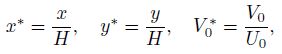
We note that, when α increases, the pressure drop and fractional absorption increase. For the further analysis, we non-dimensionalize Eqs. (30)-(33), (41), (52), and (56) by

where U₀ is the fluid velocity at the entrance of the slit. Then, we get where To study the effects of α, the uniform absorption parameter V₀, and the flow rate Q₀ on the components of the velocity, the flow rate, the pressure wall shear stress, the fractional absorption, and the leakage flux through graphs, we first remove ^* and choose the positions x = 0.1 (the entrance), x = 0.5 (the middle place), and x = 0.9 (the exit) of the slit.

The effects of α on the flow variables are depicted in Figs. 2-6. Figure 2 demonstrates the effects of α on the longitudinal velocity component u at the entrance, the middle place, and the exit when we move forward in the slit. The parabolic profile at the entrance is higher in the magnitude than those in the middle place and the exit of the slit. It is observed that, when α increases, u decreases at both the entrance and the middle place of the slit. It is noted that, when α → 0, the absorption becomes uniform throughout the slit and the magnitude of the velocity u is lower than that of linear absorption. In Fig. 3, the effects of α on the absolute transverse components of the velocity |v| are depicted. We find that, with the increase in α, |v| increases at the entrance by a small amount, comparing with those at the middle place and the exit of the slit. It is observed that, when α → 0, |v| has its highest value at all the positions in the slit. The volume flow rate, the pressure difference, and the wall shear stress decrease from the entrance to the exit of the slit. From Fig. 4, we can see that, these quantities decrease with the increase in α, and have the minimum values when α → 0. The behavior of the leakage flux q(x) is shown in Fig. 5(a), which increases with the increase in α. The streamlines are drawn for different values of α to visualize the flow behaviors (see Figs. 5 and 6). From these graphs, we can conclude that, when the magnitude of α becomes large, the adsorption (blockage) phenomenon in the kidney occurs, while in the artificial kidney, this phenomenon predicts low efficiency, resulting in more treatment time during the dialysis.

Figure 7 shows the effects of V₀ on u at the entrance, the middle place, and the exit of the slit when we move forward in the slit. It is seen that the parabolic profile at the entrance of the slit is higher in the magnitude than those at the middle place and the exit of the slit. When V₀ increases, u decreases at both the entrance and the middle of the slit. Similar effects can be observed at the exit of the slit for small values of V₀. However, a reverse flow is observed for high values of V₀ (see Fig. 7(c)). Figure 8 shows that, with the increase in V₀, the magnitude of |v| increases at the entrance, the middle place, and the exit of the slit (see Fig. 8). The volume flow rate decreases and the pressure difference increases with the increase in V₀ (see Figs. 9(a) and 9(b)). The wall shear stress decreases with the increase in V₀ (see Fig. 9(c)). Figure 10 shows the streamlines for different values of V₀. From the figure, we can see that, when V₀ → 0, the streamlines become straight, showing that there is no absorption through the walls and the forward flow is obtained.

Figures 11 and 12 show the effects of Q₀ on the longitudinal velocity and the transverse velocity at the entrance, middle place, and exit, respectively. From Fig. 11, we can see that u is parabolic and increases with the increase in Q₀ at the entrance, middle place, and exit of the slit along the x-axis. Figure 12 shows the negligible effects of Q₀ on |v|. Figure 13 shows the effects of Q₀ on the flow rate, the slit pressure difference, and the wall shear stress, respectively. Figure 14 shows the effects of Q₀ on the streams. In Fig. 13(a), the volume flow rate decreases from the entrance to the exit. With the increase in Q₀, the magnitude of the flow rate increases. From Fig. 13(b), we can see that the pressure difference decreases downstream. From Fig. 13(c), we can see that the wall shear stress at the center of the slit decreases with the increase in Q₀. From Fig. 13(c), we can study the effects of Q₀ on the wall shear stress. It is observed that the wall shear stress and the volume flow rate have the same behavior (see Figs. 13(a) and 13(c)). The effects of Q₀ on the streamlines are shown in Fig. 14. It is noted that, as Q₀ → ∞, the streamlines become straight, implying that u dominates over v.

5 Summary and conclusions

In this paper, we obtain the exact solution for the two-dimensional creeping flow through a porous slit with linear absorption. The coupled partial differential equations are transformed into a single equation in terms of the stream function. The exact solutions for the velocity profile, the volume flow rate, the pressure, the pressure drop, the wall shear stress, the fractional absorption, and the leakage flux are explicitly obtained. An important observation is that the forward flow is possible only if the volume flow rate is larger than the absorption velocity throughout the slit, otherwise all the fluid will be absorbed, which is physiologically impossible. From this work, we also observe that:

(i) The profile of the longitudinal component of the velocity at different positions is parabolic, which has the maximum value at the center or the minimum at the walls. Meanwhile, the transverse component of the velocity has the maximum value near the walls and is zero at the center.

(ii) The volume flow rate, the pressure difference, the wall shear stress, and the leakage flux decrease along the downstream direction.

(iii) When the uniform absorption velocity approaches zero, the result for the Poiseuille flow is recovered.

(iv) The pressure drop, the fractional absorption, and the wall shear stress decrease with the increase in the uniform absorption velocity.

(v) The magnitude of the longitudinal velocity decreases with the increase in the uniform absorption velocity, while the magnitude of the transverse velocity increases at all positions in the slit.

(vi) The volume flow rate increases the longitudinal velocity component, but shows negligible effects on the transverse velocity component throughout the slit.

(vii) The streamlines become straight as the absorption velocity approaches zero (simple Poiseuille flow).

(viii) The leakage flux and the fractional absorption increase with the increase in the absorp- tion parameter. The dialyzer efficiency increases if the protein adsorption at the walls decreases. Moreover, the metabolic waste can be removed from the blood by reducing the fouling (α → 0), and the treatment time during the dialysis can be reduced, which is significant physiologically.

Besides, we would like to point out here that our study is of theoretical nature and much more experimental and physiological works are needed to gain a complete insight into the flow phenomenon through renal tubule/artificial kidney.

Acknowledgements

The authors thank the reviewers for their valuable suggestions and comments.