1 Introduction

“Tensor” is defined by Gressmman. “Tensor analysis” is created by Einstein. In the opin-ion of Einstein, “tensor analysis” is the equivalent word of “Riemann geometry”, because the relativity theory is the mechanics in the Riemann space and the geometric foundation of the relativity theory is the Riemann geometry. What about the prospect of the axiomatization of the Riemann geometry? The answer is not optimistic.

Axiomatization originates from Euclid. In the elementary geometry, only two theorems belong to Euclid. However, Euclid’s greatness is his brilliant thought of axiomatization. On the basis of five axioms, he sets up the strict logic system of the geometry that can unify all the mathematical achievements in his times.

In 1935, the Bourbaki School came to being in France. Bourbaki created the concept of “mathematical structures”, in which three keywords are included, i.e., axiomatization, struc-turalization, and unification. Since then, the axiomatization thought has become a powerful tool in unifying mathematics and revealing the deep relations between different branches of mathematics. Nevertheless, some branches cannot be axiomatized and structuralized. One of them is the Riemann geometry.

Roughly speaking, the forehead of the axiomatization of the Riemann geometry is gloomy. Because of the close relations between the Riemann geometry and the tensor analysis, we may say that the possibility of the tensor analysis axiomatization is also very small.

However, there is no need to be over pessimistic. In recent years, progresses have been made in the geometrization of micro/nano mechanics^{[1, 2, 3, 4, 5, 6]}. On the basis of the axiom of the covariant form invariability, Yin^{[7, 8, 9]} extended the classical covariant derivative to the generalized covari-ant derivative. From this breakthrough point, we can see the tendency of the structuralization and unification of the tensor analysis. The possibility of axiomatization occurs.

In the tensor analysis, the two concepts, i.e., the covariant derivative and the covariant differentiation, are closely related. Therefore, this paper will focus on such a question: since the classical covariant derivative can be extended to the generalized covariant derivative, can we extend the classical covariant differentiation to the generalized covariant differentiation through axiom? If the answer is positive, then may the aximatization tendency be further strengthened?

Under the curved coordinate system in the three-dimensional (3D) flat space, the theory will be developed around two core concepts. One is the generalized components, and the other is the generalized covariant differentiation. The former is extended from the classical components, and the latter is defined from the axiom.

2 Classical covariant differentiation

Covariant differentiation originates from Christoffel^[10] and Lipschitz and Ricci-Curbastro^[11]. In 1892, Ricci-Curbastro published his “absolute differential calculus”^[10]. In 1901, Ricci-Curbastro and Levi-Civita published the summary article “methods of the absolute differential calculus and their applications”^[11]. Ricci-Curbastro’s absolute differential calculus is exactly the covariant differential calculus.

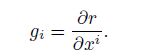
The core concept of the covariant differential calculus is the “covariant differentiation”. Under the curved coordinate system in the 3D flat space (see Fig. 1), the natural coordinate xⁱ is selected, and the natural base vector can be expressed by the point vector as follows^[12]:

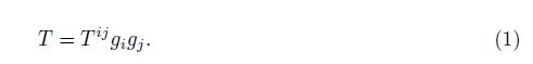
Under the curved coordinate system, the second-order tensor T may be formulated as follows:

Its common differentiation is where Then, we have where DT _^ij is the covariant differentiation of the component T _ij. Obviously, the covariant differ-entiation DT _^ij is the extension of the common differentiation dT _^ij . DT _^ij is also the component of the tensor dT .

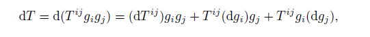
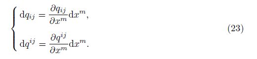
In history, Christoffel and Lipschitz mainly cared about the global differential form of the co-variant differentiation DT _^ij , while Ricci-Curbastro was more interested in the derivative inside. Ricci-Curbastro noticed that the coordinate differentiation dx^m was a quantity determined by observers, and hence should be excluded. There is

The common differentiation dT _^ij is the linear combination of the common partial derivative $\frac{\partial {{T}^{ij}}}{\partial {{x}^{m}}}$. Substituting Eq.(5) into Eq. (4), we can get two terms. One is dx^m, and the other is unrelated with dx^m.

i.e., where ∇_mT _ij , which is the term unrelated with dx^m, is the covariant derivative of the compo-nent T ^_ij of the tensor T . Its definition is^[12]

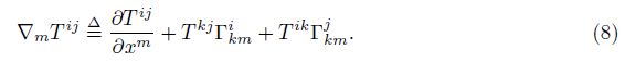
Equation (7) means that the covariant differentiation DT _^ij is the linear combination of the covariant derivative ∇_mT _ij . At this stage, the basic thought about the covariant differential calculus is formed.

Ricci-Curbastro noticed that the covariant derivative ∇_mT _ij was the component of a third-order tensor, which is coincident with his favorite judgment, i.e., components are important. Ricci-Curbastro’s tastes formulate the modern covariant differential calculus. The covariant differential calculus is exactly the differential calculus of components.

However, the components of a tensor are concepts with limitations^{[7, 8, 9]}. To break through the limitations, we need to extend the concepts and introduce the axiom.

3 From classical components to generalized components

To simplify the statement of the axiom, we introduce the concept of the generalized compo-nent.

The component T _ij in Eq. (1) is just the classical one. T _ij satisfies two fundamental trans-formations. One is the index transformation, and the other is the coordinate transformation^[12],

The coordinate transformation coefficient β_iⁱ′ is defined by

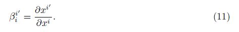
Any classical component satisfies similar fundamental transformations. In history, Ricci-Curbastro made clearly the essence of the fundamental transformations, and endowed them the core positions in the tensor analysis. Therefore, we call them the “Ricci-Curbastro transforma-tions”.

The Ricci-Curbastro transformations form two continuous transformation groups. We call them the “Ricci-Curbastro transformation groups”. All the tensors are invariants under the Ricci-Curbastro transformation groups.

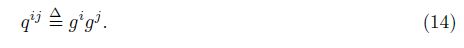
The classical components satisfy the Ricci-Curbastro transformations, but the geometric quantities satisfying the Ricci-Curbastro transformations may not be the classical components. For example, the base vector gⁱ satisfies the Ricci-Curbastro transformations, but it is not a classical component, i.e.,

Similarly, gⁱg^j satisfies the Ricci-Curbastro transformations, but it is not a classical compo-nent either. For simplification, we introduce the symbol as follows:

Its Ricci-Curbastro transformations are expressed as follows:

If we compare Eqs. (9) and (10) with Eqs. (15) and (16), respectively, we may have new discoveries. Although T _ij and q^ij are completely different concepts, they have the following common points:

(i) They are all organic parts of the tensor:

(ii) They all meet the Ricci-Curbastro transformations.

(iii) Their Ricci-Curbastro transformation groups are completely the same in forms.

Obviously, if we disregard the detailed meanings of T _ij and q^ij and only focus on the apparent forms of their Ricci-Curbastro transformations, then we can say that there is no difference between T _ij and q^ij at all. In other words, T _ij and q^ij can be considered as the same quantities.

Thus, we make the definition: any geometric quantity satisfying the Ricci-Curbastro trans-formations is termed as the “generalized component”. According to the pure formalized defini-tion, not only gⁱ and gⁱg^j but also T _ijgⁱ and T ^ijg_j are generalized components. Once the generalized component is defined, the axiom may be depicted.

4 Axiom of covariant form invariability

In Ricci-Curbastro’s covariant differential calculus, both the covariant derivative ∇_m(·) and the covariant differentiation D(·) can only act on the tensor components. These are exactly the limitations of ∇_m(·) and D(·).

To overcome the limitation of ∇_m(·), we set up the axiom of covariant form invariability, in which the concept of the generalized covariant derivative is defined by^{[7, 8, 9]}: the generalized covariant derivative of the generalized component is completely identical in the forms to the classical covariant derivative of the classical component.

This axiom extends the classical covariant derivative into the generalized covariant deriva-tive. The classical covariant derivative can only act on the classical components, while the generalized covariant derivative can act on the generalized components.

Similarly, to overcome the limitation of D(·), we will set up the axiom of covariant form invariability, in which the concept of the generalized covariant differentiation is defined by: the generalized covariant differentiation of the generalized component is completely identical in the forms to the classical covariant differentiation of the classical component.

This axiom extends the classical covariant differentiation into the generalized covariant dif-ferentiation. The classical covariant differentiation can only act on the classical components, while the generalized covariant differentiation can act on the generalized components.

The axiom of covariant form invariability for the generalized covariant derivative^{[7, 8, 9]} is very similar in content to that for the generalized covariant differentiation. In fact, in the following sections, we will prove that they are completely equivalent in essence. Therefore, they are unified as “the axiom” in the following sections.

5 Axiom-based definition of generalized covariant differentiation

This section aims at the generalized components with free indexes and their generalized covariant differentiations.

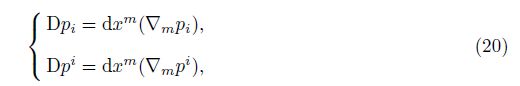
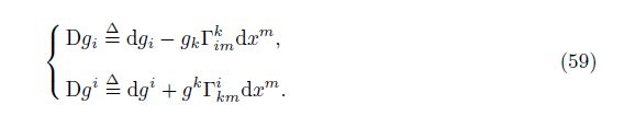
5.1 Generalized covariant differentiation of generalized component with single

index According to the axiom, the generalized covariant differentiation of the generalized compo-nent p_i or pⁱ with one free index can be defined by

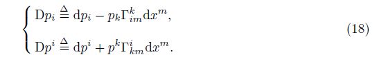
The common differentiation in Eq. (18) can be expressed as

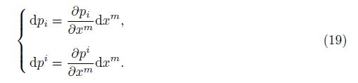
Through Eq. (19), Eq. (18), and the axiom, we can get

where^[7]

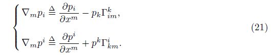
The generalized component pⁱ can be either the vector component vⁱ or the base vector gⁱ. Because pⁱ has one free index, it may be called the “1-index” generalized component.

It can be proved that both ∇_mpⁱ and Dpⁱ satisfy the Ricci-Curbastro transformations and thus they are all generalized components. Because ∇_mpⁱ has two indexes, it may be called the “2-index” generalized component. Because Dpⁱ has one index, it may be called the “1-index” generalized component.

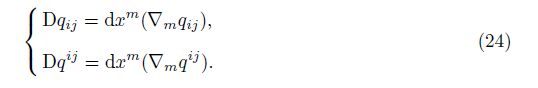
5.2 Generalized covariant differentiation of generalized component with two in-dexes

According to the axiom, the generalized covariant differentiation of the generalized compo-nent q_ij or q^ij with two free indexes can be defined by

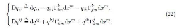
It is noted that Eq. (22) is identical in the form of Eq. (4).

The common differentiation in Eq. (22) can be expressed as

Through Eq. (23), Eq. (22), and the axiom, we can get

Here, the axiom-based definition of the generalized covariant derivative ∇_mq^ij (∇_mq_ij ) is^[7]

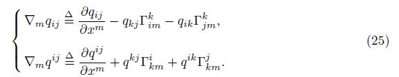
Similar to ∇_mT _ij, ∇_mq^ij satisfies the Ricci-Curbastro transformations, and it is a “3-index” generalized component. Similar to q^ij , Dq^ij satisfies the Ricci-Curbastro transformations, and it is a “2-index” generalized component.

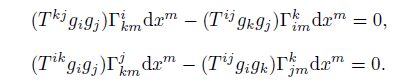
5.3 Fundamental combination mode in generalized covariant differentiation

From Subsections 5.1 and 5.2, we can say that the generalized covariant differentiation of any generalized component with a free index can be defined through the axiom of covariant form invariability.

We compare Eq. (22) with Eq. (4). Similar to the classical covariant differentiation DT _^ij , the generalized covariant differentiation Dq^ij also includes two parts. One is the common differ-entiation dq^ij , and the other is the algebraic terms q^kjΓ_kmⁱ dx^m and q^ikΓ_km^j dx^m. The common differentiation dq^ij can be expressed by the linear combination of the common partial deriva-tive $\frac{\partial {{q}^{ij}}}{\partial {{x}^{m}}}$ (see Eq. (23)). After further combination with the algebraic terms q^kjΓ_kmⁱ and q^ikΓ_km^j, the generalized covariant differentiation Dq^ij can be finally expressed by the linear combination of the generalized covariant derivative ∇_mq^ij (see Eq. (24)). This combination process is of universality, and may be called the “fundamental combination mode”.

The fundamental combination mode shows that the generalized covariant differentiation D(·) and the generalized covariant derivative ∇_m(·) are always related by

Equation (26) reveals the intrinsic relations between D(·) and ∇_m(·). It can be considered as the first-order differential form.

Equation (26) confirms the equivalence between the two axioms in Section 4. Because dx^m weights ∇_m(·) linearly, the axiom for the generalized covariant derivative ∇_m(·) is completely equivalent to that for the generalized covariant differentiation D(·).

We further pay attention to the relation between the common differentiation and the common partial derivative:

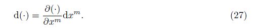
Equation (27) is valid for any generalized component, and so is Eq. (26). Equation (27) is the foundation of the classical differential calculus, while Eq. (26) is the foundation of the generalized covariant differential calculus.

There are differences between Eq. (26) and Eq. (7). In Eq. (7), the classical covariant dif-ferentiation can only act on the classical components. In Eq. (26), the generalized covariant differentiation acts on any generalized component. Therefore, Eq. (26) is much more powerful than Eq. (7). Equation (7) is the basement for the classical covariant differential calculus, and Eq. (26) is the basement for the generalized covariant differential calculus. Therefore, in com-parison with the classical covariant differential calculus, the generalized covariant differential calculus is much more powerful.

6 Leibniz rule for generalized covariant differentiation

The generalized covariant differentiation of the multiplication of a few generalized compo-nents obeys the Leibniz rule.

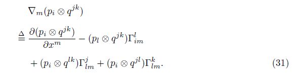
The multiplication p_i ⊗ q^jk of two generalized components can be treated as a “3-index” generalized component. Here, p_i ⊗ q^jk represents three types of multiplication, i.e., p_i · q^jk, p_i × q^jk, and p_iq^jk. According to the axiom, D(p_i ⊗ q^jk) can be defined by

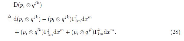
It can be proved that D(p_i ⊗ q^jk) satisfies the Ricci-Curbastro transformations and can be regarded as a “3-index” generalized component.

Equation (28) includes two combination modes. We first check the fundamental combination mode. The common differentiation can be expressed into the linear combination of the partial derivative as follows:

Combing Eq. (28) and Eq. (29), we can express the generalized covariant differentiation into the linear combination of the generalized covariant derivative as follows:

Here, the axiom-based definition of the generalized covariant derivative ∇_m(p_i ⊗ q^jk) is^[7]

Then, we concentrate on the first combination mode in Eq. (28). The first combination mode includes the following operations.

Apply the Leibniz rule to the common differentiation in Eq. (28) as follows:

With Eq. (32), Eq. (28), and the axiom, we can obtain the multiplication formula of the generalized covariant derivative as follows:

showing that D(p_i ⊗ q^jk) obeys the Leibniz rule.

7 Generalized covariant differentiation of generalized components with dummy indexes

This section will define the generalized covariant differentiation of the generalized compo-nents with dummy indexes.

We check T ^ijg_j , which is a part of the second-order tensor T . T ^ijg_j can be understood in two ways. One is that there is one free index in T ^ijg_j , and thus can be regarded as a “1-index” generalized component. In this case, the axiom-based definition of D(T ^ijg_j) is

The other is that there is one free index and a pair of dummy indexes inside T ^ijg_j . Both the dummy indexes satisfy the Ricci-Curbastro transformations. Therefore, T ^ijg_j can be considered as a “3-index” generalized component. In this case, the axiom-based definition of D(T ^ijg_j) is

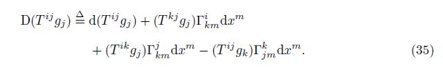
However, is there any contradiction between Eq. (34) and Eq. (35)? The answer is “no”. The reason is as follows.

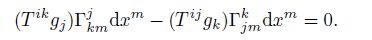
Different from D(p_i ⊗ q^jk), D(T ^ijg_j) includes three types of combination modes. Except the fundamental combination mode and the first combination mode, there is the second combination mode, which may be operated as follows. Combing the last two terms in Eq. (35), we can get

Therefore, Eq. (35) and Eq. (34) coincide completely with each other.

D(T ^ijg_j) satisfies the Ricci-Curbastro transformations, and can be regarded either as a “1-index” generalized component or a “3-index” generalized component.

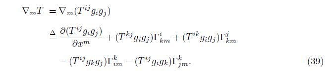
8 Generalized covariant differentiation of tensor

A tensor is an objective quantity. We check the tensor T with the rank two. T can be understood as follows. First, T is an invariant under the Ricci-Curbastro transformation groups, and thus it is also a generalized component. Second, there are two pairs of dummy indexes inside T . Each dummy index satisfies the Ricci-Curbastro transformations. Therefore, T can be treated as a “4-index” generalized component. Last, the number of the free indices inside T is zero, and thus T may be treated as a “0-index” generalized component.

If T is treated as a “4-index” generalized component, then DT can be defined through the axiom as follows:

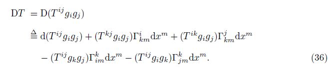
There are three combination modes in Eq. (36). We first check the fundamental combination mode. The common differentiation in Eq. (36) can be expressed as the linear combination of the common partial derivative as follows:

With Eq. (37), Eq. (36), and the axiom, we can obtain DT as follows:

Here, the axiom-based definition of the generalized covariant derivative ∇_mT is^[7]

Then, we look at the first combination mode. Apply the Leibniz rule to the common differentiation in Eq. (36), i.e.,

Then, with Eq. (36), Eq. (40), and the axiom, we can get

showing that the generalized covariant differentiation obeys the Leibniz rule.

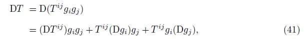
Last, we focus on the second combination mode. Keep the common differentiation in Eq. (36) unchanged, and combine the algebraic terms in pairs, i.e.,

Then, Eq. (36) can be degenerated into leading to the proposition as follows: the generalized covariant differentiation of the tensors is equal to its common differentiation.

Equation (42) can be regarded as the definition formula for the generalized component T with “0-index”.

DT is an objective quantity. It can be treated both as a “4-index” generalized component and a “0-index” generalized component.

9 Generalized covariant differentiation of multiplication of tensors

We check the tensor B = B_ijgⁱg^j , the vector C = C_kg^k, and their multiplication B⊗C, i.e.,

which can be treated as a “6-index” generalized component. According to the axiom, D(B ⊗ C) can be defined by which includes three combination modes. We first check the fundamental combination mode. The common differentiation in Eq. (44) can be expressed as the linear combination of the com-mon partial derivative as follows: With Eq. (45), Eq. (44), and the axiom, we can get the linear combination of the generalized covariant derivative as follows:

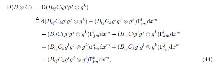
Here, the axiom-based definition of the generalized covariant derivative ∇_m(B⊗C) is^[7]

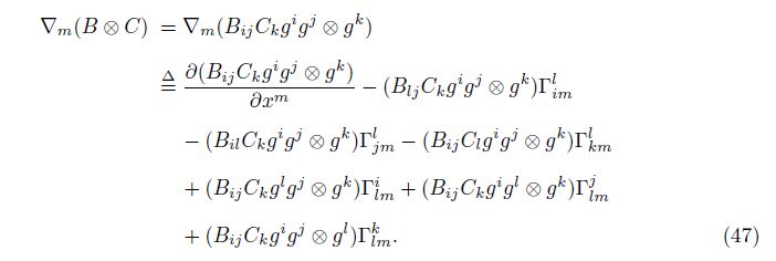
Then, we look at the first combination mode. Apply the Leibniz rule on the common differentiation in Eq. (44), i.e.,

With Eq. (44), Eq. (48), and the axiom, we can get

showing that the generalized covariant differentiation obeys the Leibniz rule.

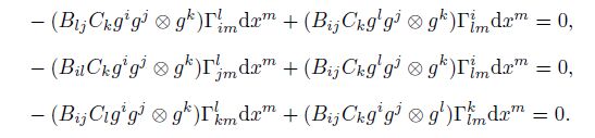
Finally, we concentrate on the second combination mode. Keep the common differentiation in Eq. (44) unchanged, and combine the algebraic terms in pairs, i.e.,

Then, Eq. (49) becomes which is the extension of Eq. (42). B ⊗C can be globally considered as a “0-index” generalized component. Its generalized covariant differentiation is equal to its common partial differentia-tion.

10 Generalized covariant differentiation of square root of determinant of metric tensor

The square root of the determinant of the metric tensor G = g_ijgⁱg^j is $\sqrt{g}$. Its definition formula is

which can be considered as a “3-index” generalized component. According to the axiom, D$\sqrt{g}$ can be defined by which also includes three combination modes. We first check the fundamental combination mode. The common differentiation in Eq. (52) can be expressed as the linear combination of the common partial derivative as follows: With Eq. (52), Eq. (53), and the axiom, we can rewrite the generalized covariant differentiation as the linear combination of the generalized covariant derivative as follows:

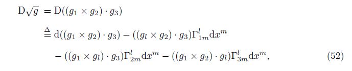
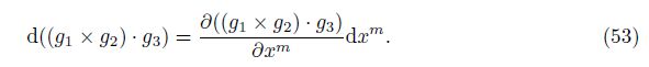
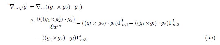
Here, the axiom-based definition of the generalized covariant derivative ∇_m$\sqrt{g}$ is^[7]

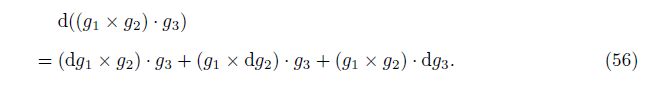
Then, we look at the first combination mode. Apply the Leibniz rule to the common differentiation in Eq. (52), i.e.,

With Eq. (52), Eq. (56), and the axiom, we can get showing that the generalized covariant differentiation obeys the Leibniz rule.

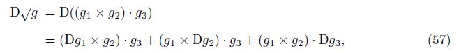
Finally, we concentrate on the second combination mode. Keep the common differentiation in Eq. (52) unchanged, and combine the algebraic terms in pairs, i.e.,

Then, Eq. (50) can be rendered to the following form:

11 Algebraic structure of generalized covariant differentiation

The axiom of covariant form invariability endows the algebraic structure to the generalized covariant differentiation.

From the definition formula mentioned above, it may be concluded that the summation operation of the generalized covariant differentiation is of completeness. From the Leibniz rule in the first combination mode, it may be concluded that the multiplication operation of the generalized covariant differentiation is of completeness.

Thus, the set of the generalized covariant differentiation with complete summation and multiplication will form the “ring”. We may say that the algebraic structure of the generalized covariant differentiation is a “covariant differential ring”.

Obviously, the generalized covariant differentiation D(·) and the generalized covariant deriva-tive ∇_m(·) have an identical algebraic structure^[7]. This is not strange. The transformation in Eq. (26) assures that the algebraic structures of D(·) and ∇_m(·) must be the same.

Now, we can make the prediction that there are two ways, i.e., the indirect way and the direct way, to calculate the generalized covariant differentiation D(·).

The indirect way is to calculate D(·) through ∇_m(·) (see Eq. (26)). The direct way is to calculate D(·) directly through the covariant differential ring. In this case, an essential problem should be solved: how do we calculate the generalized covariant differentiation of the base vector?

12 Covariant differential transformation group

In Eq. (18), let p^m = g^m. Then, the generalized covariant differentiation of the base vector can be defined by

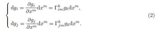
From Eq. (2) or the following formulations:

Eq. (59) can be rewritten as follows:

The generalized covariant differentiation of the base vector is always zero. Although the base vector changes from point to point, it can get in or get out of the generalized covariant differentiation D(·), just as a constant vector in appearance.

Up to now, the generalized covariant differentiation of the base vector is not only definable but also calculable under the curved coordinate system.

Similar to Ref. ^[7], Eq. (61) defines the continuous differential transformation group. We also call it the “covariant differential transformation group” under the curved coordinate system.

The covariant differential transformation group in Eq. (61) is essentially equivalent to that in Ref. ^[7]. This equivalence is proved as follows. According to the fundamental combination mode, Eq. (61) will lead to

From Eq. (62), we can obtain that the necessary and sufficient condition for the validity of Eq. (61) is

which is exactly the covariant differential transformation group in Ref. ^[7].

13 Extremely simple calculations of generalized covariant differentiation

The covariant differential transformation group in Eq. (61) assures that the generalized co-variant differentiation of any generalized component is calculable. Besides, the 0 in Eq. (61) leads to the extreme simplicity in the calculation of the generalized covariant differentiation. This simplicity can be seen from the proposition that the generalized covariant differentiation of any generalized component calculated from the algebraic operations of the base vectors is always 0. The detailed examples are listed as follows.

The decomposition formula of the metric tensor is G = g_ijgⁱg^j . From Eq. (61), we can get

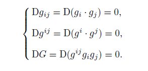
These results show that g_ij , g^ij , and G can get into or get out the generalized covariant differentiation D(·) freely.

The decomposition formula of the Eddington tensor is

The component is

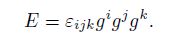
According to Eq. (61), we have

These results show that ε_ijk, ε^ijk, and E can get into or get out the generalized covariant differentiation D(·) freely.

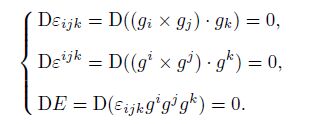
In the textbook, very complicated calculations are necessary to derive the above results. Now, their correctness becomes obvious under the generalized covariant differentiation and the covariant differential transformation group.

14 Some interesting results

Under the covariant differential transformation group, some interesting results may be derived.

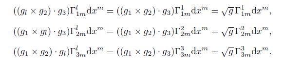
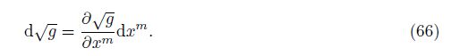
With the axiom, we can define the generalized covariant differentiation of $\sqrt{g}$ by Eq. (25). However, Eq. (25) is only a definition formula, and it is not the calculation formula. To calculate D$\sqrt{g}$, we must make use of the covariant differential transformation group. From Eq. (61), we may obtain

The generalized covariant differentiation of $\sqrt{g}$ is always 0. Hence, $\sqrt{g}$ can get into or get out D(·) freely. This is a beautiful property.

Combining Eq. (64) and Eq. (58), we may derive

which may lead to the formulations below. From the fundamental combination mode, d$\sqrt{g}$ can be expressed as the linear combination of the partial derivative as follows:

With Eq. (66) and Eq. (65), we can get

leading to

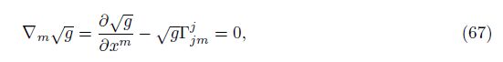
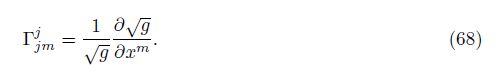
Equation (68) is the classical result in the tensor analysis.

Now, we pay attention to the last equality in Eq. (65), i.e.,

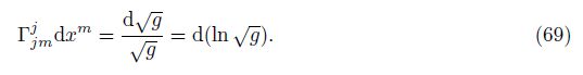
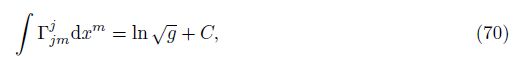
Integrating Eq. (69) on both sides, we have

which can also be obtained from Eq. (68).

15 Conclusions

The progresses in this paper can be summarized as four concepts or thoughts, i.e., the Ricci-Curbastro transformation, the generalized component, the generalized covariant differentiation, and the axiom of covariant form invariability. Their logic relations may be described as fol-lows: the Ricci-Curbastro transformation is the origin from which the generalized component is abstracted. The generalized component constrains the objectives on which the generalized covariant differentiation can act. The generalized covariant differentiation is regulated by the axiom of covariant form invariability. On the bases of the generalized covariant differentia-tion and the covariant differential transformation group, the differential calculus in the tensor analysis is extremely simplified.

Bourbaki’s thought (axiomatization, structuralization, and unification) is still valid in the tensor analysis. Under the axiom of covariant form invariability, the covariant differential cal-culus in the tensor analysis is unified as a whole. In other words, the axiomatization of the absolute differential calculus developed by Ricci-Curbastro can be realized, and the generalized covariant differential calculus can be established.