�?span class="paragraph_title outline_anchor" level="1">1 Introduction

Fractional differential equations have attracted considerable attention in recent years due to their applications in physics^[1],geology^{[2, 3]},biology^[4],chemistry^[5],and finance^[6]. However,few explicit analytical solutions for fractional differential equations are available. Therefore,numerical methods become the major means to solve fractional differential equations^{[7, 8, 9, 10, 11, 12, 13, 14, 15, 16, 17, 18]}.

In recent years,some efficient numerical methods have been considered by many authors. Zheng et al.^[19] derived a high order space-time spectral method,employing the Jacobi polynomials for the temporal discretization and the Fourier-like basis functions for the spatial discretization for the time fractional Fokker-Planck initial-boundary value problem. Shen et al.^[20] studied the finite difference methods for the non-linear fractional diffusion/wave diffusion equations with a variable order time-fractional derivative operator. Liu et al.^[21] developed a novel weighted fractional finite volume method based on the nodal basis functions for the two-sided space fractional diffusion equation,and pointed out that this method could be extended to twodimensional and three-dimensional problems with complex regions. Feng et al.^[22] proposed a fractional finite volume method for the two-sided space fractional diffusion equation based on the nodal basis functions,and proved that the derived numerical scheme was unconditional stable and convergent. Liu et al.^[23] considered a meshless scheme based on the radial basis functions for a fractal mobile/immobile transport model. Liu et al.^[24] developed two meshless schemes based on the point interpolation method for the one-dimensional space fractional diffusion equation. Feng et al.^[25] proposed a Crank-Nicolson scheme for the one-dimensional space fractional diffusion equation with a variable coefficient,and proved that the numerical scheme was unconditional stable and convergent with the second-order accuracy. Liu et al.^[26] derived a novel alternating direction implicit method for the two-dimensional Riesz space fractional diffusion equation with a non-linear reaction term. Yang et al.^[27] established a finite volume scheme with the preconditioned Lanczos method as an attractive and high-efficiency approach for the two-dimensional space fractional reaction-diffusion equations.

The fractional percolation equation (FPE),which is a mathematical model for the seepage flow problems in groundwater and fluid dynamics in porous media^{[28, 29, 30]},is a partial differential equation obtained from the traditional percolation equation^[31] by replacing the space integer derivatives by the space fractional derivatives. A three-dimensional FPE is proposed by He^[32] as follows:

where 0 < α_i < 1,0 < β_i �?1,and i = 1,2,3. p = p(x,y,z,t) is the pressure. K_x,K_y,and K_y are the percolation coefficients along the x-,y-,and z-directions,respectively. f(x,y,z,t) is the source term. v is the velocity. is the percolation domain.

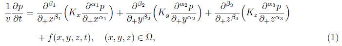
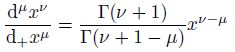
The space fractional partial derivatives in (1) are defined in the Riemman-Liouville form. Generally,for any μ > 0,the Riemann-Liouville fractional derivative $\frac{{{d}^{\mu }}u(x)}{d+{{x}^{\mu }}}$of the order μ is defined by^{[33, 34, 35]}

where n is an integer,and n�? < μ �?n. If μ is an integer,then (2) gives the standard integer derivative.

In the FPE (1),we denote the rate of the fluid mass flux q = (q_x,q_y,q_z),where

It should be pointed out that the expression (3) is derived from the modified Darcy law proposed by He^[32] and Ochoa-Tapia et al.^[36] for describing the solute movement in a non-homogeneous porous medium. Notice that the continued seepage flow leads to β_i = 1 (i = 1,2,3) while (1) models a rigid body motion where β_i = 0 (i = 1,2,3). However,the reality is that the seepage flow is neither continuous nor rigid. Therefore,0 < β_i < 1 is more general. Under this consideration,He^[32] proposed an approximate analytical solution for (1) by the variational iteration method. In the numerical aspect,Chen et al.^[37] developed an implicit finite difference method for the one-dimensional FPE. Chen et al.^[38] considered an alternating direction implicit difference method for the two-dimensional case. Chen et al.^[39] discussed the numerical simulation of the two-dimensional variable-order FPE. Liu et al.^[40] proposed two finite difference methods for the three-dimensional non-continued seepage flow problem with constant percolation coefficients and the continued seepage flow problem with variable percolation coefficients,respectively.

In Refs. ^[37]-^[40],the FPEs are studied with the Dirichlet boundary conditions. As we all know,in seepage flow problems,the Robin boundary condition

represents the linear replenishment or percolation of the fluid mass flux on the boundary ∂Ω ,where γ> 0,and n is the outward unit normal. The Neumann boundary condition is used to describe the variation of the fluid mass flux q on ∂Ω. Notice the modified Darcy law (3),if we consider the corresponding Robin or Neumann boundary condition for the FPE (1),then the fractional derivative of the pressure p will be employed in the boundary expressions,which may be characterized as fractional boundary conditions.

Recently,Jia andWang^[41] considered the space fractional diffusion equations with fractional derivative boundary conditions,and developed fast implicit finite difference methods for both steady-state and time-dependent problems. To our knowledge,the study on the numerical computation of FPEs with fractional derivative boundary conditions is still limited. This motivates us to examine an implicit finite difference method for the one-dimensional FPE with fractional Robin/Neumann boundary conditions in this paper.

The rest of the paper is organized as follows. In Section 2,we construct an implicit finite difference method,and analyze its consistency. In Section 3,we study the unconditional stability and convergence of the method in two cases. In Section 4,we carry out numerical experiments to verify the accuracy and efficiency of the proposed scheme. Finally,we draw our conclusions in Section 5.

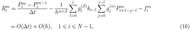
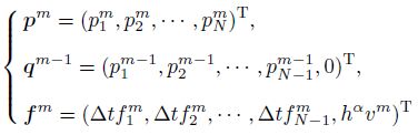
2 Implicit finite difference method and its consistency

In this section,we discuss the following simplified one-dimensional fractional percolation problem with the left-sided mixed fractional spatial derivative as follows:

where γ= 0 corresponds to a fractional Neumann boundary condition,and γ> 0 corresponds to a fractional Robin boundary condition.

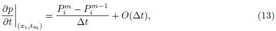
Let h = L/N and △t = T/M be the spatial mesh-width and the time step,respectively,where N and M are positive integers. We define a spatial partition by x_i = ih (i = 0,1,...,N) and a temporal partition by t_m = m△t (m = 0,1,... ,M). Let

Denote the exact and numerical solutions at the mesh point (x_i,t_m) by P _i^m = p(x_i,t_m) and p_i^m ,respectively. The initial and the Dirichlet boundary conditions are set by p_i⁰ = p₀(x_i) and p₀^m = 0,respectively.

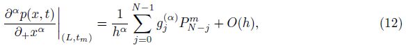
To approximate the left-sided mixed fractional spatial derivative,Chen et al.^[37] defined the operator �?sub>h,q^α,β as follows:

where q is a non-negative integer,and g_j^(α) = (�?)^j 􀀀(_j^α ) in which α and j are the fractional binomial coefficients. It is proved that ^[37] which is uniform for x �?(0,L) as h �?0 under the assumption of the homogenous Dirichlet boundary condition on x = 0. Thus,for q = 1,the left-sided mixed fractional spatial derivative in (6) can be approximated as follows: where Using the standard left Grünwald-Letnikov fractional derivative^[10] to approximate the left-sided fractional derivative of the order α in the fractional boundary condition on x = L,we have where 1 �?m �?M. We employ the backward Euler scheme to approximate the first-order time derivative and present an implicit finite difference scheme as follows: Denote the local truncation error by R_i^m for 1 �?i �?N. Then,from (11)-(13),we have This implies the consistency of the implicit finite difference scheme above both the interior nodes and the right boundary node.

3 Stability and convergence analysis

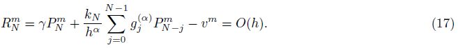
In this section,we discuss the stability and convergence of the numerical method under two special cases,i.e.,a continued seepage flow (β = 1) with a monotone percolation coefficient k(x) and a seepage flow with the fractional Neumann boundary condition (γ= 0).

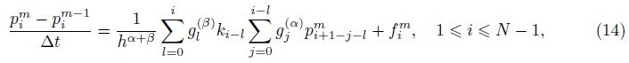
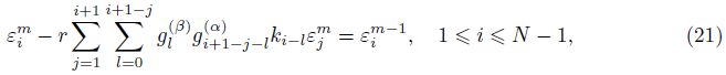
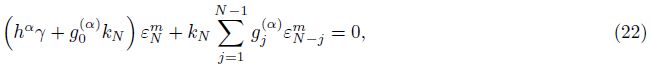
Let $r = {{{\rm{t}}} \over {{h^{\alpha + \beta }}}}$ be the mesh ratio. Then,we rewrite (14) by exchanging the order of the summation as follows:

Denote the column vectors as follows: for 1 �?m �?M. Then,the matrix form of the implicit finite difference schemes (14) and (15) can be expressed as where the coefficient matrix A = (a_i,j )_i,j=1^N and its entries are

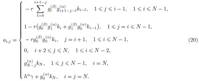
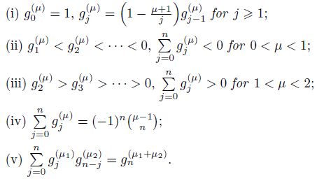
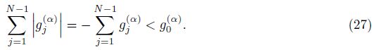
Some properties of the alternating fractional binomial coefficients g_j^(α) and g_l^(β) in (20) are listed in the following lemma^[34].

Lemma 1  Let μ,μ₁, and μ₂ be positive real numbers,and the integer n �?1. We have

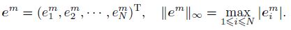
To discuss the stability of the numerical method,we denote by $\tilde{p}_{i}^{m}$ the approximate solution of the difference scheme with the initial condition$\tilde{p}_{i}^{0}$ ,where 1 �?i �?N and 1 �?m �?M,and define

For the convergence analysis,we define and From the definition of the finite difference scheme,we have where ε₀^m = 0 (m = 1,2,... ,M). Recalling (16) and (17),we have where e₀^m = 0 (m = 1,2,... ,M),and e_i⁰ = 0 (i = 0,1,... ,N).

Now,we give the following stability and convergence theorem under the assumption of continuity of the seepage flow (β = 1).

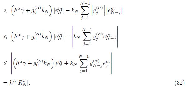
Theorem 1  If β = 1,γ> 0,and k(x) decreases monotonically with respect to x in [0,L],then the implicit finite difference scheme (19) is unconditional stable,and there exists a positive constant C independent of △t and h such that

Proof  For β = 1,we have g₀ ^(β) = 1,g₁^(β) = �?,and g_j^(β) = 0 (j �?2). The entries in the first (N �?1) rows of the matrix A can be rewritten as follows: where 1�?i �?N �?1. By Lemma 1,we have Taking the monotonicity of k(x) into consideration,when 1 �?i �?N �?1,we have It follows from (22) that Therefore,we suppose that${{\left\| {{\varepsilon }^{m}} \right\|}_{\infty }}=\left| \varepsilon _{{{i}_{0}}}^{m} \right|$,where 1 �?i₀ �?N �?1. Then, which implies that Thus,the numerical method defined by (19) is unconditional stable with respect to the initial data.

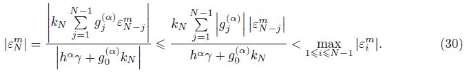
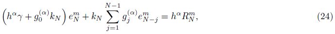
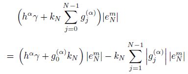
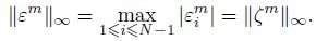
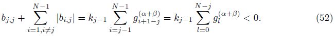
For 1 �?m �? M,if ${{\left\| {{e}^{m}} \right\|}_{\infty }}=\left| e_{N}^{m} \right|\ge \underset{1\le i\le N-1}{\mathop{\max }}\,\left| e_{i}^{m} \right|$,it follows from (24) that

With Lemma 1 and the Stirling formula for the Gamma function^[25],we have as N �?�? Combining (32) and (33),we get If then

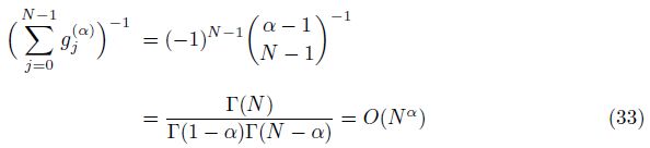
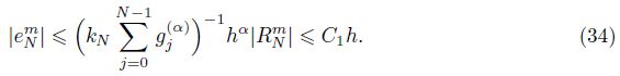
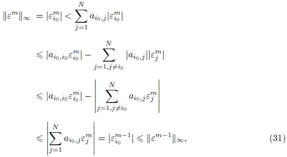
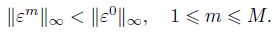
By induction,we can finally obtain

This completes the proof.

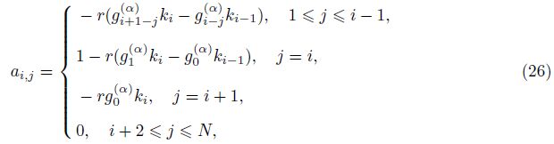
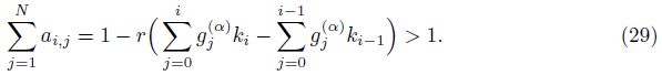
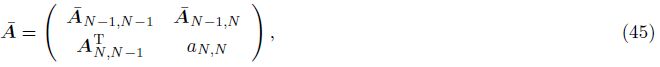
Before proceeding to the case with the fractional Neumann boundary condition ( γ= 0),let us consider a equivalent form of the finite difference scheme (19). We express the coefficient matrix A defined by (20) in a block form as follows:

where A_N�?,N�? is the (N �?1)-by-(N �?1) matrix that consists of the first (N �?1) rows and the first (N �?) columns of A,A_N�?,N is an (N �?)-dimensional column vector that consists of the first (N �?1) entries in the Nth column of A,and A _N,N�?^T is an (N �?1)-dimensional column vector that consists of the first (N �?1) entries in the Nth row of A.

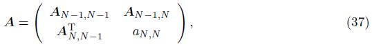
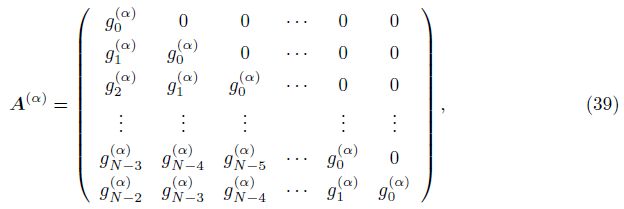
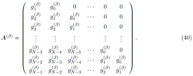
It is simple to show that the matrix A_N�?,N�? has the following decomposition:

where I is the identity matrix of the order N �?1,c_N�? is the (N �?1)th column of I,k = (k₀,k₁,... ,k_N�?)^T,g^(α) = (g_N�?^(α) ,g_N�?^(α) ,... ,g₁^(α) )^T,and A^(α) and A^(α) are (N �?)-by-(N�?) Toeplitz matrices^[42] defined by According to the definition (20),we can write A_N�?,N and A_N,N�?^T as follows: Let${{\omega }_{N}}=\frac{r{{k}_{N-1}}}{{{k}_{N}}}$. Notice that a_N,N = h^α γ+ k_Ng0^(α) . Let ω_N time the Nth equation to the (N �?)th equation in the linear system (19). Then,we get a equivalent form of (19) as follows: where For the stability of the numerical method under the assumption thatγ = 0,we have the following theorem.

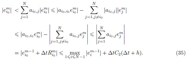
Theorem 2  If 1 < α + β < 2 and γ= 0,then the implicit finite difference scheme (19) is unconditional stable.

Proof  Let

Notice that γ= 0 leads to A_N�?,N = 0. Then,we can rewrite (21) and (22) as follows: Similar to the inequality (30) in Theorem 1,from (49),we have This means that Since it suffices to prove that the spectral radius of the matrix ( A_N�?,N�?)^�? is less than one.

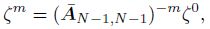
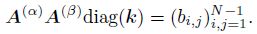
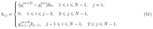
Our first goal is to show that the eigenvalues of the matrix A^(α)A^(β)diag(k) have negative real parts. Denote

It follows from Lemma 1 that the entries b_i,j have the following form: According to the Gerschgorin theorem^[43],the eigenvalues of the matrix A^(α)A^(β)diag(k) lie in the union of the disks centered at b_j,j with the radius$\sum\limits_{i=1}^{N-1}{\left| {{b}_{i,j}} \right|}$. We observe from Lemma 1 that b_j,j < 0 and b_i,j > 0 for all i �?j. When 2 �?j �?N �?1,we have For j = 1,we compute The two inequalities (52) and (53) imply that all of the Greschgorin disks of the matrix A^(α)A^(β)diag(k) are within the left half of the complex plane. Thus,the eigenvalues of the matrix A^(α)A^(β)diag(k) have negative real parts.

Next,by the fact that

we have that A_{N�?, N�?} has the same eigenvalues with I �?r ( A^(α)A^(β)diag(k)) . Thus,each eigenvalue of A_N�?,N�? has a magnitude larger that 1. Therefore,the spectral radius of the matrix 􀀀(A_N�?,N�? )^�? is less than 1. This completes the proof.

Remark 1 Under the assumption of Theorem 2,although a convergence estimate such as (25) is not given,some numerical experiments in Section 4 show that the implicit finite difference scheme defined by (19) is also temporally and spatially first-order accurate.

4 Numerical examples

We present two numerical examples for solving the initial-boundary value problem of (6)-(8) by the implicit finite difference method given in Section 2. Denote ${{\left\| e_{h}^{M} \right\|}_{\infty }}$ the maximum error of the numerical solution at the time t = T for �?i>t = h. Let ${{G}_{h}}={{\log }_{2}}({{\left\| e_{2h}^{M} \right\|}_{\infty }}/{{\left\| e_{h}^{2M} \right\|}_{\infty }})$reflect the convergence order of the method. All numerical experiments are run in MATLAB on a Thinkpad E420 laptop with the following configuration: Intel(R) Core(TM) i3-2350M CPU 2.30GHZ and 4GB RAM.

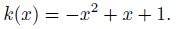
Example 1  We solve the initial-boundary problem (6) with the following data. The spatial domain is [0,L] = ^{[0, 1]},and the time interval is [0,T] = ^{[0, 1]}. The percolation coefficient is

It is obvious that k(x) decreases monotonically with respect to x in ^{[0, 1]}. The exact solution of this problem is which satisfies the homogenous Dirichlet boundary condition on x = 0. The initial condition is The source term f(x,t) and function v(t) may be obtained by substituting the exact solution into (6) and its fractional Robin boundary condition (7) withγ= 1 by using the formula for the Riemann-Liouville fractional derivative.

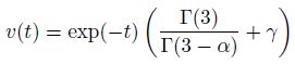
Example 2  In this example,set the spatial domain [0,L] = ^{[0, 1]},the time interval [0,T] = ^{[0, 1]},and the percolation coefficient

The fractional boundary condition and the initial condition are and p₀(x) = x²,respectively. The source term is where α,β�?(0,1). The exact solution of this problem is p(x,t) = exp(�?i>t)x².

In our numerical experiments,we consider three different α in each case,respectively. Table 1 shows the maximum errors at the time T = 1 for Example 1,where γ = 1 and β = 1.0,it illustrates the stability and the O(�?i>t) + O(h) convergence rate of the implicit finite difference scheme (19) proved in Theorem 1. The error data obtained at the time T = 1 for Example 2,where γ = 0 and β = 0.8,are reported in Table 2,which reflects the stability of the numerical method and supports Theorem 2. In Table 3,the error data at the time T = 1 for Example 2,where γ = 1 and β = 0.8,are given. It is observed from Tables 2-3 that the numerical method is also temporally and spatially first-order accurate for the non-continued seepage flow with the fractional Neumann or Robin boundary condition. This implies that the stability and convergence condition in Theorems 1 and 2 can be weakened.

5 Conclusions

In this paper,an implicit finite difference method is developed for the one-dimensional FPE with the Dirichlet and fractional boundary conditions. The unconditional stability and convergence of the method are proved for two cases,i.e.,a continued seepage flow with a monotone percolation coefficient and a seepage flow with the fractional Neumann boundary condition. The numerical experiments illustrate the practicability of the numerical scheme. Numerical methods for the two- or three-dimensional FPEs will be considered in our future work.

Acknowledgements

The authors would like to express their sincere thanks to the referees for their valuable comments and suggestions which helped to improve the original paper. The authors are also grateful to Dr.Yongqiang LYU of Shandong Normal University for his helpful suggestions.