 2016, Vol. 37
Shanghai University
Article Information
- Long ZHU, Xiang QIU, Jianping LUO, Yulu LIU. 2016.
- Scale properties of turbulent transport and coherent structure in stably stratified flows
- Appl. Math. Mech. -Engl. Ed., 37(4): 443-458
- http://dx.doi.org/10.1007/s10483-016-2043-9
Article History
- Received Apr. 15, 2015;
- in final form Sept. 1, 2015


2. School of Science, Shanghai Institute of Technology, Shanghai 201418, China;
3. Shanghai Institute of Applied Mathematics and Mechanics, Shanghai University, Shanghai 200072, China
Turbulence in the oceans and atmosphere are usually stably stratified in density due to vertical salinity and temperature gradients. The dynamics of stratification,which leads to qualitative and quantitative vertical scalar transport driven by buoyancy,is known to exhibit very particular phenomena,i.e.,gradient transport and counter-gradient transport (CGT) in experimental,numerical,and theoretical studies. The issue of scalar transport in stably stratified turbulent flows is not only interesting from a fundamental point of view but also a key to understand mixing and dynamical processes in environmental or engineering problems.
One of the fundamental characteristics of turbulence is that it has stronger transport than laminar flows. The gradient transport assumption is used in most of the turbulent models to assume that the scalar fluxes are transported towards the direction in which the mean quantities decrease. However,it is well known in laboratory and engineering that the CGT phenomena appear[1, 2] which cannot be described by the Fourier law. For example,there is a region in the channel where the heat flux $\overline {{u_i}\theta } $ and the mean temperature gradient ${{\partial \Theta } \over {\partial {x_j}}}$ have the same sign, i.e.,$\overline {{u_i}\theta } {{\partial \Theta } \over {\partial {x_j}}}$ > 0,which means that the heat is counter-gradiently transported[3].
The CGT phenomena were first found in laboratory in the stratified open channel flow by Komori et al.[4]. Thereafter,the problem of freely decaying turbulence,especially the CGT phenomena in the flow,has already been extensively studied in laboratory experiments,for instance,the grid-turbulence experiments of Huang and Schmitt[5],Lohse and Xia[6],Chandra and Verma[7],and Demars and Manson[8] and the wind tunnel experiments of Keller and Atta[9]. The first direct numerical simulation (DNS) of homogeneous turbulence in the stratified shear flow was performed by Gerz et al.[10]. Following that study,there were a lot of research works with numerical simulation by Matheou and Chung[11] and Bartello and Tobias[12]. Also,Kumar and Dewan[13] and van Hooff et al.[14] performed a large eddy simulation (LES) study of the uniform stably stratified shear flow.
In the previous studies,researchers believed that the complexity of stratified turbulence arises from the coexistence of two timescales,i.e.,the turnover timescale,which is associated with the eddy structures,and the buoyancy timescale,which is associated with the buoyancy acting on the fluid particles. Currently,it is well known that the major effect of the buoyancy forces is to reduce the vertical kinetic energy and the vertical turbulent transport,leading to the formation of vertical patches separated by strong horizontal vortex sheets,which was testified by laboratory experiments and numerical simulation. Fincham et al.[15] gave the first clear experimental evidence,which showed that the dissipation in the stratified turbulent flow is mainly controlled by the local horizontal velocity. In the most strongly stratified flows,one striking phenomenon is the oscillation in time of the buoyancy turbulent vertical flux between positive and negative (counter-gradient) values[16, 17]. It was found that the vertical buoyancy flux not only oscillates as time evolves but also remains persistently counter-gradient for large time.
For a long time,the turbulent CGT is regarded as one of the fundamental causes of turbulence, especially for the strong dissipative complex system[18]. Although the research on mechanism of the CGT has continued,many results show the upon homologous conclusion. In the previous studies,we can conclude that coherent structures may be one of the important causes of the CGT. Therefore,the target for the later investigation can be details about interactions between different scales of eddies at different temporal and spatial positions. To this end,different analytical methods,including the Fourier analysis,the wavelet analysis[18, 19],the proper orthogonal decomposition (POD)[20, 21],and the empirical mode decomposition (EMD)[22, 23], which were introduced to analyze the turbulence signal,have provided different promising tools to catch different principal properties in turbulence. The EMD is the latest one used to analyze turbulence time series[15, 24].
A motivation of this study is that the former studies on the CGT in stratified turbulence seldom considered the contribution of small scales to turbulent transport,particularly to the turbulent scalar CGT,and the EMD provides a good method to decompose turbulence signals into different modes (scales) to examine the contributions from different scales. The turbulence time series in this study is traced by the LES[25, 26].
In the following sections,the computational domain from the physical model is introduced, and some important parameters are given. In Section 3,the EMD method is introduced in detail to see how we can decompose nonlinear signals and its advantages in analyzing turbulence signals. The turbulent CGT properties are discussed in Section 4. The intermittency and the probability density function (PDF) on the modes are shown in this section. The coherent structures in the streamwise velocity and the vertical velocity have different time scales. Section 5 summarizes the conclusions on the turbulence properties of CGT in a stably two-layerstratified flow.
2 PhysicalmodelThe schematic diagram of the computational domain of grid-generated turbulent stratified flow is the same as the model in Ref. [25]. The computational domain is 1.02 m×0.1 m×0.1 m (51 m×5 m×5 m) in the streamwise,vertical,and span wise directions. A square turbulencegenerating grid,on which the velocity components are set to zero,is located at 0.02 m downstream from the entrance. The mesh size M and the diameter of the round rod d are 0.02 m and 0.002 2 m,respectively. A clapboard of 0.002 m thickness is placed between the entrance and the grid to separate hot and cold water coming from the inlet. The non-slip conditions are adopted for the upper,lower,and side boundaries. The number of the meshes is about 1 970 000.
In this model,the entrance is set as two different streams. The mean velocities of the upper and lower streams are set to be the same value of 0.125 m/s. The distribution of temperature T (z) is set to depend on different runs. There are two conditions,including the temperature difference 0 K and 10 K and the velocity difference 0.05 m/s. In order to compare with different conditions,the Reynolds number based on the length of grid and the mean velocity between the upper and lower layers is fixed to be 2 500.
The two computational runs,respectively,are Sh (the mean velocity 0.125 m/s and the velocity difference 0.05 m/s) and St (the mean velocity 0.125 m/s,the velocity difference 0.05 m/s, and the temperature difference 10 K). Sh is neutral stratification,and St is strong stratification. In data analysis,the EMD is used to the streamwise velocity,the vertical velocity,and the temperature of runs of Sh and St in different positions. In this paper,we show the results of the positions x/M = 6,x/M = 12,and x/M = 40 at the centerline (M = 0.02 m). The steamwise velocity is u,the vertical velocity is v,and the temperature is T .
3 EMDThe process of channel flow is mostly nonlinear and non-stationary,exhibiting the coexistence of different time scales. The EMD is an effective tool which analyzes nonlinear and non-stationary time sequences by a series of intrinsic mode functions (IMFs) to analyze nonlinearities considered as fast oscillations and low frequency. It is without a priori basis,unlike the traditional Fourier-based method and wavelet transform. The high frequency can be recognized as an IMF,and the lower one is the residual. The IMF can satisfy two conditions,that is,(i) the number of local extrema is different,and the number of zero in time series must be zero or one; (ii) the running mean value of the envelop estimated by the local maxima is zero.
The EMD is based on the following assumptions: (i) the time series signal has at least two extrema: one maximum and one minimum; (ii) the characteristic time scale is regulated by the time lapse between the extreme values; (iii) if the signals are entirely devoid of extrema but contained only inflection points,then the extrema can be revealed through differentiating the EMD one or more times. Final consequences can be acquired by integration(s) of components.
The EMD algorithm is designed to extract the IMF modes as follows:
(i) Identify the local extrema which contain the maxima and minima points for a given time series θ(t).
(ii) A cubic spline algorithm constructs the upper envelop emax(t) (the extremum maxima) and the lower one emin(t) (the extremum minima) for the local maxima and local maxima, respectively.
(iii) The definition of the mean m1(t) between these two envelops is

(iv) The first component is defined by

(v) Ideally,h1(t) can be an IMF as expected,if h1(t) complies the above-mentioned conditions to IMF’s respects. In reality,however,h1(t) may not. Then,h1(t) is taken as a new time sequences,and this sifting process is repeated j times until h1j(t) is an IMF,

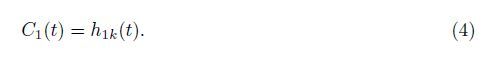
The first IMF component C1(t) is
The first residual r1(t)

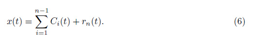
When rn(t) becomes a monotonic function or a constant,the shifting procedure is not repeated at all. Finally,the original signal θ(t) can be decomposed into n - 1 IMF modes and one residual rn(t).
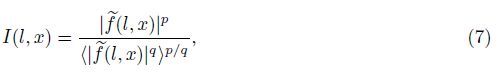
As we know,intermittency is the most principal factor which causes certain turbulent quantities away from the Gaussian distribution. However,the mechanism of intermittency remains open. There are many different ways to describe the intermittent events. The local intermittency is mainly considered here. Farge[27] gave his description of intermittency as follows:
Figures 1-4 show the different modes of streamwise velocity,vertical velocity,and temperature signal decomposed with the EMD method (see Fig. 1(a)),local intermittency (see Fig. 1(b)),and probability density distributions (see Fig. 1(c)) in runs of St at the position x/M = 6. In research,we choose x/M = 6,x/M = 12,and x/M = 40,three different positions in runs of Sh and St. The EMD method,the local intermittency,and the probability density distributions are the same as the results in Fig. 1 to Fig. 4,which are not shown in this paper.C1,C2,· · · ,C10 denote different modes from the EMD,and Roou is the residual of output. Comparing Fig. 1 with Fig. 4,the streamwise velocity time series of shear flows can be decomposed into more modes. It means that the velocity time series of shear flows contain more different time scale coherent structures. The intermittency in stratified flows is stronger than that in shear flows, especially in high frequency modes.

|
| Fig. 1 Intermittency and PDF on modes of run of St (position x/M = 6 and instantaneous velocity u) |

|
| Fig. 2 Intermittency and PDF onmodes of run of St (position x/M = 6 and instantaneous velocity v) |

|
| Fig. 3 Intermittency and PDF on modes of run of St (position x/M=6 and instantaneous temperature T) |

|
| Fig. 4 Intermittency and PDFon modes of run of Sh(position x/M=6 and instantaneous temperature T) |
Figure 1(a) clearly shows that the energy of the first-order only takes a small part of the whole mean energy,but it occupies a majority of mean energy in the second-order,which indicates that the streamwise velocity fluctuation is mainly in the second modes. The same results from the vertical velocity can be summarized in other figures. It is noticed that modes mixing occurs in the decomposition,because of the effects of singular events. The method in Ref. [20] has to be used to get rid of the singular events. Also,there is an interesting phenomenon that the double peak values in the first-order of PDF occur in most cases. One of the possible reason is the choice of sub-grid scale in the LES,and usually the first-order modes denote the background noise in turbulence. Another possible reason is rested with the turbulence itself,but the same phenomena at the smallest scale have not been found before.
In Fig. 1(b),there is a stronger intermittency in smaller scales,considering the PDFs of different modes in Fig. 1(c),except for only few modes subjected to the Gaussian distribution. It departs from the Gaussian distribution in almost all of the modes. Also,we find interesting phenomena that there are double peak values in the first-order of PDF in streamwise and vertical velocities. One of the possible reason is the choice of sub-grid scale in the LES. Usually, the first-order modes denote the background noise in the turbulence. Another possible reason is rested with the turbulence itself,but we cannot find the same phenomena at the smallest scale before.
Comparing the results among different signals,we find that the modes which show the strong intermittency from the streamwise velocity are more than the vertical velocity and temperature, and the strong intermittency of streamwise velocity distributes in more modes. Also,the results in different positions show that with the evolution of the flow,the intermittency becomes weaker, but it spreads to more modes.
4.2 Coherent structureAs we know,turbulence is dominated by the coherent structure. Traditionally coherent structure is distinguished from how much energy it contains,for instance,through the methods of VITA,POD,and wavelet analysis. Similarly,in the EMD method,the coherent structure is also recognized in the sense of mean energy. It considers that if the mean energy in the mode exceeds 10% of the whole fluctuation energy,the mode is the coherent structure mode. The reason we choose different values of energy ratio to estimate the coherent structure is that we still can give a complete explanation to the complicated process of generation and evolution of coherent structure until now.
Tables 1 and 2 show the mean energy and its corresponding mean period in different modes of streamwise and vertical velocity of run of Sh using the EMD. As far as Table 1 is concerned, for the streamwise velocity,there are three modes,modes 6,7,and 8,in which the mean energy is over 10%,and the total energy contained in these three modes accounts for 84.89% of the total energy. Their mean periods are 0.489 6 s,0.938 4 s,and 2.326 4 s,respectively. For the vertical velocity,there are two modes of 3 and 4 exceeding 10%. They contain 97.76% energy of the total,and the corresponding periods are 0.361 2 s and 0.673 4 s,respectively.


Tables 3,4,and 5 show the mean energy and its corresponding mean period in different modes of streamwise and vertical velocity of run of St using the EMD. As far as Table 3 is concerned,for the streamwise velocity,there are four modes,modes 5,6,7,and 8,in which the mean energy is over 10%,and the total energy contained in these three modes accounts for 86.95% of the total energy. Their mean periods are 0.114 7 s,0.162 4 s,0.288 8 s,and 0.571 4 s,respectively. For the vertical velocity,there are three modes of 2,3,and 4 exceeding 10%. They contain 88% energy of the total,and the corresponding periods are 0.139 3 s,0.169 8 s,and 0.269 8 s,respectively. There is a significant difference between the coherent structure of streamwise velocity and vertical velocity,based on the former study. We know that it is resulted from the anisotropy of the stratified field. For the temperature signal,we just consider the square of the fluctuations as the denotation of energy,which may not make any sense physically. From the results,we find that the main modes of energy containment are in lower modes.


There are different mean time scales of coherent structure between the streamwise velocity and the vertical velocity,and it shows the anisotropy of stratified turbulent field. Coherent structures play a principal role in the stratified turbulence with the development of the flow, and the energy is distributed to more modes with the effects of stratification.
Concluding from Fig. 5,the mean period of modes in runs of Sh and St have a linear relation on the semilog coordinate. In Fig. 5,the mean period of the streamwise velocity and the vertical velocity has the analogical longest and shortest periods. However,the streamwise velocity has more modes than the vertical velocity. This means that the components in period of the streamwise velocity are more complicated. We can conclude that the streamwise fluctuating intensities are larger than the vertical fluctuating intensities. Figure 6 shows the same consequence.

|
| Fig. 5 Mean period of modes of u and v in run of Sh, which illustrates estimated mean period versus mode in log-linear plot |

|
| Fig. 6 Mean period of modes of u and v in run of St, which illustrates estimated mean period versus mode in log-linear plot |
Figures 5 and 6 illustrate the estimated mean frequency ωn versus the mode index n in a log-linear plot. An exponential decrease is observed and modeled by a relation in the form of ωn = ω0η-n. For the mean frequency of the streamwise velocity in run of Sh,there are ω0 $ \simeq $ 0.002 6 Hz and η = 2.356 3 obtained using a least square fitting algorithm in the range 1 $ \ll $ n $ \ll $ 8. The mean frequency ωn of modes n is 2.356 3 times larger than the next one.ω0 $ \simeq $ 0.036 4 Hz and η = 2.071 1 are calculated by the mean frequency of vertical velocity in run of Sh,and the analogical results are obtained in run of St. This characteristic corresponds to an almost dyadic filter bank property of the EMD algorithm.
4.3 Turbulent scalar CGTThe turbulent CGT phenomenon has been introduced in the first section of this paper. In this part,we will study the turbulent scalar CGT in detail.
We find that the evolution of vertical heat flux on the centerline is along the vertical velocity direction,and it is normalized by the product of the root mean square of fluctuating velocity and temperature. The consequence shows that the vertical heat flux decreases along the flow direction. The reason is that with the development of the stratified turbulence,the mixing of the two layers is more enhanced,which leads to the decrease of the vertical density gradient. Therefore,the vertical velocity fluctuation is depressed.
Because the flow is stable (considered in this study),the vertical temperature gradient is positive in the field,${{\partial \Theta } \over {\partial {x_j}}}$> 0. However,there exists a small zone of x/M < 10,in which the vertical heat flux is negative,$\overline {v\theta } $> 0. Thus,we receive $\overline {v\theta } {{\partial \Theta } \over {\partial {x_j}}}$> 0,which means that in this area,turbulent counter gradient heat transport occurs.
In the former research of fully developed asymmetric channel flow using the wavelet analysis[23],through analyzing the wavelet cross-spectrum of Reynolds stress,the consequence shows that local CGT exists at some scales,while gradient transport exists at other scales. In the CGT region,the sum of contributions from those scales that exhibit local CGT is more than that of contributions from those scales that exhibit gradient transport. In this part,when the EMD method is used to decompose the velocity signal into several components of different scales,the transport properties of different scales also show CGT phenomena.

|
| Fig. 7 Local vertical heat flux in corresponding modes (run of St), which illustrates local CGT phenomena at certain modes, while gradient transport occurs at other modes |
Based on the results of previous research,we calculate that turbulent heat CGT occurs at the position x/M = 6($\overline {{u_i}\theta } {{\partial \Theta } \over {\partial {x_j}}}$> 0) in run of St,but does not occur at the positions x/M = 12 and x/M = 40. Figure 6 shows the contributions of the modes of vertical velocity to vertical heat flux at x/M = 6,x/M = 12,and x/M = 40. It is shown from Fig. 6 that local heat CGT occurs at different modes,but the global heat CGT,which is the integration of local CGT in all modes,is different in the three positions. Concretely,global heat CGT appears at the position of x/M = 6,but at the position of x/M = 12 and x/M = 40,the heat transport is gradient transport. This result agrees with the former analysis consequence.
Table 6 shows the contribution of different modes to the vertical heat flux in detail. The values are obtained by multiplying 100 to the original value,where the value of zero denotes that the contribution of the mode is very small.

About the vertical heat flux,one point is confirmed obviously that the local heat flux transport also contains positive and negative values in each model. This suggests that the gradient and counter gradient compete with each other in the local heat flux of every model. The whole transport needs to consider comprehensively with the local heat flux of each model.
Table 7 shows the principal mode of coherent structure and the principal mode on which the contribution to vertical heat flux is dominating. We can find that the principal modes under the two different meanings are almost consistent with each other,that is,the stratified turbulence is dominated by coherent structures. Of course,the other modes also contribute to the heat flux,but they are not primary compared with those certain principal modes.

In the present work,the velocity and the temperature of stratified turbulence from the LES are analyzed with the EMD. The signals are decomposed into different modes to study the scale characteristics of the intermittency,the coherent structure,and the turbulent CGT.
It shows that the turbulent statistics depart from the Gaussian distribution at most of the modes. The velocity intermittency is suppressed along the downstream,and it is scattered to more modes. The intermittency is intensified by the stratification in small scales.
There are different time scales of coherent structure in different modes between the streamwise and vertical velocities. It means that the stratified turbulent field is anisotropic. The coherent structures play a principal role in the turbulent heat transport in stratified flow. With the development of the flow,the turbulent kinetic energy is distributed to more modes with the effects of stratification.
The analysis of vertical scalar transport shows that there are local CGT phenomena at certain modes,while gradient transport occurs at other modes. However,there is also the global counter-gradient scalar transport resulting from the total contributions of all modes on the CGT,and the modes of coherent structures are consistent with the modes which contribute to the vertical scalar transport principally including gradient and counter-gradient cases.
| [1] | Jiang, J. B., Liu, Y. L., and Lu, Z. M. Experimental and theoretical studies on negative transport phenomena in turbulent flows. Advances in Mechnics, 30(2), 1-8(2000) |
| [2] | Kolmogorov, A. N. The local structure of turbulence in an incompressible viscous fluid for very large Reynolds numbers. Proceedings of the Royal Society of London, 434, 9-13(1991) |
| [3] | Eskinazi, S. and Yeh, H. An investigation of fully developed turbulent flows in a curved channel. Journal of the Aeronaut Sciences, 23, 23-31(1956) |
| [4] | Komori, S., Ueda, H., Ogino, F., and Mizushina, T. Turbulence structure in stably stratified open-channel flow. Journal of Fluid Mechanics, 130, 13-26(1983) |
| [5] | Huang, Y. X. and Schmitt, G. Analysis of experimental homogeneous turbulence time series by Hilbert-Huang transform. 18éme Congrés Francais de Mécanique, 18, 27-31(2007) |
| [6] | Lohse, D. and Xia, K. Q. Small-scale properties of turbulent Rayleigh-Benard convection. Annual Review of Fluid Mechanics, 42, 335-364(2010) |
| [7] | Chandra, M. and Verma, M. K. Dynamics and symmetries of flow reversals in turbulent convection. Physical Review E, 83, 067303(2011) |
| [8] | Demars, B. O. L. and Manson, J. R. Temperature dependence of stream aeration coefficients and the effect of water turbulence:a critical review. Water Research, 47, 1-5(2013) |
| [9] | Keller, K. H. and Atta, C. W. V. An experimental investigation of the vertical temperature structure of homogeneous stratified shear turbulence. Journal of Fluid Mechanics, 425, 1-29(2000) |
| [10] | Gerz, T., Schumann, U., and Elghorashi, S. E. Direct numerical simulation of stratified homogenous turbulent shear flows. Journal of Fluid Mechanics, 200, 563-594(1989) |
| [11] | Matheou, G. and Chung, D. Direct numerical simulation of stratified turbulence. Physics of Fluids, 24, 091106(2012) |
| [12] | Bartello, P. and Tobias, S. M. Sensitivity of stratified turbulence to the buoyancy Reynolds number. Journal of Fluid Mechanics, 725, 1-22(2013) |
| [13] | Kumar, R. and Dewan, A. URANS computations with buoyancy corrected turbulence models for turbulent thermal plume. International Journal of Heat and Mass Transfer, 72, 680-689(2014) |
| [14] | Van Hooff, T., Blocken, B., Gousseau, P., and van Heijst, G. J. F. Counter-gradient diffusion in a slot-ventilated enclosure assessed by LES and RANS. Computers and Fluids, 96, 63-75(2014) |
| [15] | Fincham, A. M., Maxworthy, T., and Spedding, G. R. Energy dissipation and vortex structure in freely decaying, stratified grid turbulence. Dynamics of Atmospheres and Oceans, 23, 155-169(1996) |
| [16] | Riley, J. J., Metcalfe, R. W., and Weissman, M. A. Direct numerical simulations of homogeneous turbulence in density stratied fluids. AIP Conference Proceedings, 76, 79-112(1981) |
| [17] | Kimura, Y. and Herring, J. R. Energy spectra of stably stratified turbulence. Journal of Fluid Mechanics, 698, 19-50(2012) |
| [18] | Jiang, J. B., Qiu, X., and Lu, Z. M. Orthogonal wavelet analysis of counter gradient transport phenomena in turbulent asymmetric channel flow. Acta Mechanica Sinica, 21(2), 133-141(2005) |
| [19] | Plata, M., Cant, S., and Prosser, R. On the use of biorthogonal interpolating wavelets for largeeddy simulation of turbulence. Journal of Computational Physics, 231(20), 6754-6769(2012) |
| [20] | Lam, K. M. Application of POD analysis to concentration field of a jet flow. Journal of Hydroenvironment Research, 7(2), 171-181(2013) |
| [21] | Aranyi, P., Janiga, G., Zahringer, K., and Thevenin, D. Analysis of different POD methods for PIV-measurements in complex unsteady flows. Journal of Heat and Fluid Flow, 43, 204-211(2013) |
| [22] | Huang, N. E., Shen, Z., and Long, S. R. The empirical mode decomposition and the Hilbert spectrum for nonlinear and non-stationary time series analysis. Proceedings of the Royal Society A, 454, 903-995(1998) |
| [23] | Huang, N. E., Shen, Z., and Long, S. R. A new view of nonlinear water waves:the Hilbert spectrum. Annual Review of Fluid Mechanics, 31, 417-437(1999) |
| [24] | Huang, Y. X., Schmitt, F. G., Lu, Z. M., and Liu, Y. L. An amplitude-frequency study of turbulent scaling intermittency using empirical mode decomposition and Hilbert spectral analysis. Europhysics Letters, 84, 1-10(2008) |
| [25] | Qiu, X., Zhang, D. X., and Lu, Z. M. Turbulent mixing and evolution in a stably stratified flow with a temperature step. Journal of Hydrodynamics, 21(1), 84-92(2009) |
| [26] | Qiu, X., Huang, Y. X., and Lu, Z. M. Large eddy simulation of turbulent statistical and transport properties in stably stratified flows. Applied Mathematics and Mechanics (English Edition), 30(2), 153-162(2009) DOI 10.1007/s10483-009-0203-x |
| [27] | Frage, M. Wavelet transform and their applications to turbulence. Annual Review of Fluid Mechanics, 232, 469-478(1992) |