1 Introduction

The existence of a low velocity layer in the half-space of the Earth was established by Gutenberg^{[1, 2]}. He discovered that there exists a wave that is nothing but horizontally polarized surface waves of shear type or a Love type wave of long periods (60 s-300 s). Thus,the wave was named as the G-type seismic wave. Long chains of waves dispersed with large amplitudes were observed on Seismograms of distant surface earthquakes,and this dispersion is easily caught as first arrivals corresponding to the waves of longer periods. For these long period waves like G-type,the dispersion curve is practically flat with a velocity of 4.4 km/s and has an almost impulsive form^{[3, 4, 5, 6]},because the Love wave has a constant phase velocity of 4.4 km/s over a period of 40 s to 300 s,and their waveform is rather impulsive. We can better think of G-type with the period of 60 s-300 s. After a devastating earthquake,a chain of G-waves can be observed as it takes about two and a half hours for G-waves to travel round the globe. The long period waves mainly propagate through mantle. Thus,they are also known as mantle waves.

Experimental and theoretical investigation aiming to gain a better understanding of the real Earth has led to a requirement for more practical representation of various media through which seismic waves propagate. Therefore,in the present paper,a better realistic approach is considered by assuming a rigid boundary plane on the Earth’s crustal layer. The dispersion of seismic waves is highly affected by the elastic properties of the substratum’s materials. Moreover, the composition of the layers might be inhomogeneous and isotropic in nature or may be orthotropic,monoclinic,or any other anisotropic medium. The dispersion equation of the phase and the group velocity of the surface wave thus relies on the characteristics of the medium. Thus, these studies allow the estimate of the structure along their trajectories. Many scientists have given their immense contribution in the study of shear wave dispersion in an elastic medium by taking constant or variable velocity,rigidity,and density into account. Aki^[7] worked on Niigata earthquake and explained the generation and propagation of G-waves,while Chattopadhyay^[8] demonstrated the generation of G-type seismic waves. Chattopadhyay and Keshri^[9] explained the impact of initial stress on G-type seismic waves. Recently,Chattopadhyay and Singh^[10] worked on reinforced media and explained the propagation characteristic of G-type wave in such a medium. Yoshida^[11] explained how a dent across the continental crust contributes in the fluctuation of the group velocity of Love waves. Manna et al.^[12] studied propagation of Love wave in a piezoelectric layer over an inhomogeneous elastic half-space,whereas Singh^[13] studied the influence of Love wave in irregular boundary surfaces. Recently,Lei et al.^[14] described theoretically shear horizontal (SH) wave propagation in the periodically-layered piezomagnetic structure. The possibility of Love wave dispersion under the condition of linearly varying porosity and rigidity was investigated by Gupta et al.^[15]. Gupta and Vishwakarma^[16] explained remarkably the P and S wave propagation in an initially stressed gravitating half-space.

It is seen that the effect of rigid boundary on propagation of G-type seismic wave in a layer remains untouched. Therefore,this paper investigates the effect of rigid plane on the propagation behavior of G-waves. Inside the Earth,a very hard layer (also known as “rigid”) is present. It is a surface where the particles are not likely to displace under any external forces. Since the Earth is inhomogeneous in its composition due to the presence of a very hard layer, the heterogeneous material and the rigid surface play a remarkable role in the dispersion of the seismic waves. We consider a specific variation of the exponential type and the periodic type in the layer and the half-space,respectively. With these variations,the governing system of equation of motion has been reduced to Hill’s equation with the periodic coefficient which is then solved by the method described in Ref. ^[17]. Valeev^[17] took into consideration a certain class of system of linear differential equations with coefficients which are periodic in nature and preserve the property that by the help of Laplace transformation,they may be transformed to a system of linear difference equations,which further may be solved by the method of infinite determinants. We obtain the Laplace transform of the displacement by considering the terms up to the first-order. Finally,the phase velocity and the group velocity are obtained in a closed form,and the graphs are plotted to show the remarkable effect of the inhomogeneity,the initial stress,and the rigid boundary plane.

2 Geometry of problem

The geometry of the problem consists of a non-homogeneous crustal layer of the Earth of a finite thickness H resting over an inhomogeneous half-space under the influence of the initial stress. The upper boundary plane of the crustal layer is kept rigid,as shown in Fig. 1. A rigid surface is one where the movement of the particle is restricted and the displacement of the wave vanishes. The heterogeneity in the layer and the half-space is considered in rigidity and density. The origin of the coordinate system (x,y,z) is located at the interface,which separates the layer from the half-space,the x-axis is horizontal,and the positive z-axis is directed vertically downward,as shown in Fig. 1.

The heterogeneity in the layer and the half-space is considered as follows.

In the layer,

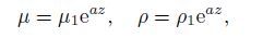
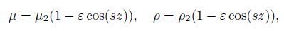
And in the half-space,

where a is a constant called the inhomogeneity parameter,and its dimension is the same as that of the reciprocal of length,ε is a small positive constant,and s is a depth parameter.

3 Solution of problem

As the shear type waves propagate horizontally and G-type waves are horizontally polarized surface waves (here along the x-axis),the displacement components u along the x-direction and w along the z-direction vanish,and only v = v(x,z,t) along the y-direction exists.

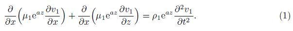
Therefore,the governing equation of motion for the upper heterogeneous layer is

In the inhomogeneous half-space under the initial stress,the displacement v₂(x,z,t) satisfies the differential equation where P is the initial stress parameter.

In the given problem,the stresses and the displacements are continuous at the interface, and the upper layer is assumed to be rigid. The boundary conditions may be written as

Now,with the help of separation of variables,we may substitute v₁(x,z,t) = V₁(z)e^ik(x-ct) in Eq. (1). Then,we obtain

where m₁²= k²(${{{c^2}} \over {{\beta ^2}}}$-1),β₁ =$\sqrt {{{\mu 1} \over {\rho 1}}} $,and ω = kc,in which k is the wave number,and c is the phase velocity.

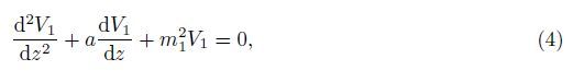
Again,putting V₁(z) = V (z)e^{-${a \over 2}$z} in Eq. (4),we get

where n₁² = m²-${{{a^2}} \over 4}$.

Therefore,we have

The upper surface is rigid in nature. Hence,using the boundary condition (3a),we get

Hence,substituting Eq. (7) in Eq. (6) yields

Now,assume Substituting Eq. (9) in Eq. (2),the equation of motion for the inhomogeneous mantle may be written as This is the differential equation which may be further solved using the method given by Valeev^[17]. We apply the Laplace transformation with respect to z,that is,we multiply Eq. (10) by e^-rz and integrate it with respect to z from 0 to ∞. Then,we get Using the boundary condition (3b),we get Now,we consider q(0) =$\left( {{{d{V_2}} \over {dz}}} \right)$z=0 and μ₂⁽⁰⁾ = μ₂(1 - ε). Then,using the boundary condition (3c),we obtain Define the Laplace transformation of V₂(z) as Using Eqs. (13)-(14) in Eq. (11),we obtain where Now,in order to find F(r) from Eq. (15),we replace r by r+ism and then divide the whole equation by (ism)ⁿ (m ≠ 0). We obtain the following infinite system of linear algebraic equations in the quantities F(r + ism) (m = 0,±1,±2,±3,· · ·), where r may be regarded as a parameter in the coefficients. Now,in order to deal with the special case m = 0 separately,we may include Eq. (15) in Eq. (17) by agreeing to regard (ism)^-n = 1 when m = 0. Solving Eq. (16),we obtain F(r) as the ratio of two infinite determinants,viz, where The first approximation of Eq. (18) is where B₁ = R₀(sin(nH)),and B₂ = R₀μ₁(n cos(nH) -${a \over 2}$sin(nH)).

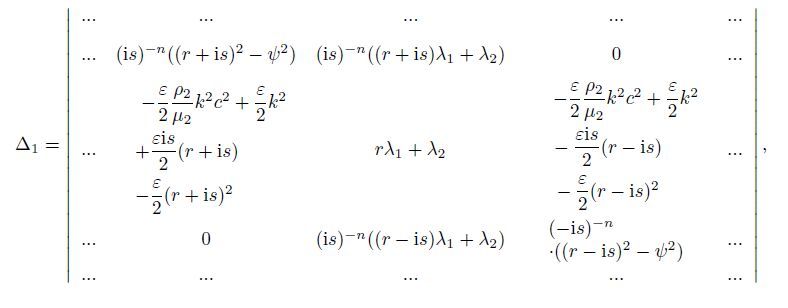
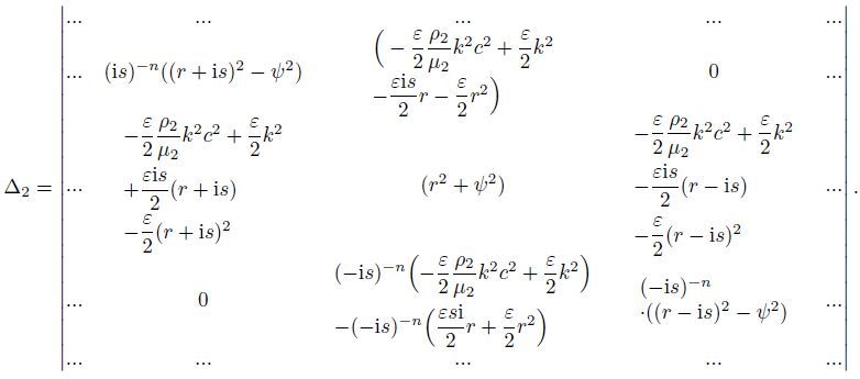
The second approximation of Eq. (19) is

where Ignoring the terms which contain ε2 and higher powers,we get Hence,Eq. (20) transforms to Then,V₂(z) may be given according to the inversion formula as The residues R₁,R₂,and R₃ at the poles r = ψ,r = ψ + is,and r = ψ - is may be presented, respectively,by where A₁ =${{\rho 2} \over {\mu 2}}$k²c² - k².

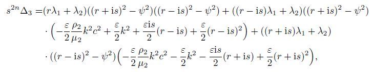
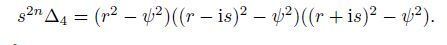
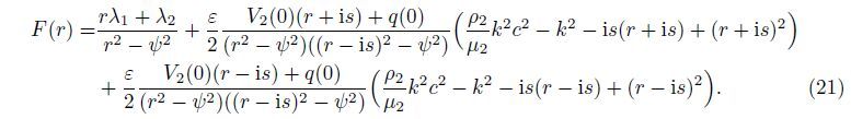
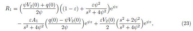
Equations (23)-(25) represent the situation for a large amount of energy remaining confined near the surface,which are

Now,Eqs. (26) and (27) give where β₁² =${{{\mu 1} \over {\rho 1}}}$,and β₂² =${{{\mu 2} \over {\rho 2}}}$.

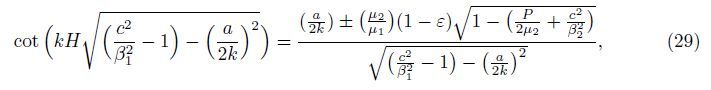
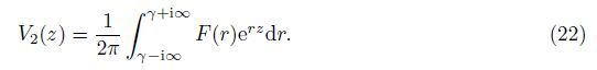
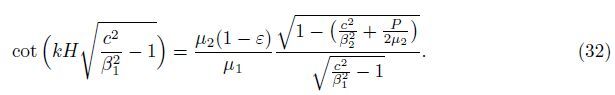
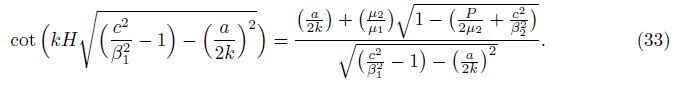
Equation (29) gives us the dispersion equation (or the frequency equation) for propagation of the G-type wave in a heterogeneous layer overlying a heterogeneous half-space under the initial stress. However,we focus only on the positive sign for further discussion.

Now,from Eq. (28),we have

Then,the group velocity U may be given by

4 Particular cases

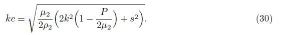
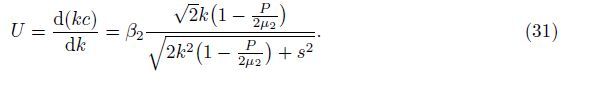
Case 1 The upper layer is free from inhomogeneity,i.e.,a = 0. Then,Eq. (31) is reduced to

This is the dispersion equation for the G-type wave in a homogeneous layer overlying a heterogeneous half-space under the influence of rigid boundary plane.

Case 2 For the heterogeneous medium lying over a homogeneous half-space,that is,for ε = 0 under the initial stress,Eq. (29) changes to

Equation (33) gives the dispersion equation of G-wave when there is no inhomogeneity in the half-space.

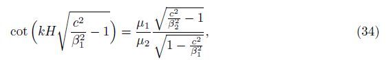
Case 3 For the layer and the half-space being free from any kind of inhomogeneity and initial stress,i.e.,a = 0,ε = 0,and P = 0,Eq. (29) converts to the general dispersion equation of Love waves,

which is the usual dispersion equation for Love waves in a homogeneous medium over a homogeneous half-space with β1 < c < β₂.

5 Numerical calculations,graphs,and discussion on results

In order to see the influence of the rigid boundary,the inhomogeneity parameter,and the initial stress on the phase velocity of G-wave,we use the dispersion relation (29). Keeping the numerical value${{{\mu 1} \over {\rho 1}}}$ = 0.02,${{{\mu 2} \over {\rho 2}}}$= 0.2,and ${{{\mu 2} \over {\mu 1}}}$= 0.1,Figs. 2-9 are plotted. Figures 2-4 signify the variation of the phase velocity against the wave number,while Fig. 5 shows the variation of the group velocity against the wave number. Figures 6-9 are surface plots drawn to demonstrate the variation more promptly.

In Fig. 2,a study has been made on the variation of inhomogeneity parameter associated with the rigidity and density of the crustal layer. The values considered for ${P \over {2\mu 2}}$ and ε are 0.6 and 0.4,respectively. It is found that the phase velocity diminishes as the wave number increases for all the values of a/k ,while at a particular wave number,the phase velocity of G-wave increases as the value of inhomogeneity increases at a particular wave number. The curves are equally apart with the equal curvature,which shows a periodic effect due to the influence of rigid boundary plane.

Figure 3 is plotted to show the impact of compressive initial stress in the half-space on the propagation of G-wave. The values of ${a \over {2k}}$ and ε are kept as 0.2. In the presence of rigid boundary plane,it is found that when there is no initial stress,the phase velocity is the minimum,while it increases as the initial stress starts existing with the increasing magnitude. The equally spaced curves in the figure show the remarkable effect of initial stress on the phase velocity of G-wave.

Similarly,Fig. 4 reveals the effect of ε on the propagation characteristic of G-wave. The values for ${P \over {2\mu 2}}$ and ${a \over {2k}}$ are 0.2 and 0.1,respectively. The patterns of G-waves are found the same as in Figs. 2 and 3,but the curves are now reversed appearing accumulating when the wave numbers are the maximum. Here,at a particular wave number,as the value of ε increases,the phase velocity of G-wave decreases. The effect may be claimed to be most likely due to the rigid boundary plane at the top.

Figure 5 is drawn for the dimensionless group velocity against the dimensionless wave number to find the impact of varying initial stress on it. It is clearly observable in the figure that the group velocity is remarkably affected when the variation in the initial stress is considered. The curvatures are sharp for all the curves. It can be concluded that the group velocity increases promptly as the wave number increases,while the group velocity decreases as the initial stress increases at a particular wave number.

Figures 6-9 are the surface plots between the group velocity U,the wave number k,and the parameter s. Figure 6 is plotted for ${P \over {2\mu 2}}$ = 0.0,Fig. 7 for ${P \over {2\mu 2}}$= 0.1,Fig. 8 for ${P \over {2\mu 2}}$= 0.2,and Fig. 9 for ${P \over {2\mu 2}}$= 0.3. The surface plot being self explanatory shows that the effect of initial stress is prominent on the group velocity under the influence of rigid boundary plane. The deviations of the surface edge are clearly visible in the entire figure showing the effect.

6 Conclusions

The dispersion equation of the phase and group velocities of G-waves is found when the crustal layer and the half-space exhibit inhomogeneity in rigidity and density that varies exponentially and periodically along the depth inside the Earth. It is observed that the rigid boundary plane plays a significant role not only in the phase velocity of G-waves but also in the group velocity which are responsible for a large amount of energy confined near the Earth’s surface. Various graphs are plotted to show the propagation pattern of G-wave. The influence of inhomogeneity presented in the rigidity and density plays a significant role in fluctuating the propagation of G-waves in the Earth crust.

The study of surface wave such as G-waves has its possible usage and application in the broad field of geophysics and in understanding the estimate and cause of damage that takes place during an earthquake.

Acknowledgements The authors thank Professor Yue LIU for his invitation of visit to University of Texas,Arlington.