 2016, Vol. 37
Shanghai University
Article Information
- Zhaodong DING, Yongjun JIAN, Liangui YANG.
- Time periodic electroosmotic flow of micropolar fluids through microparallel channel
- Appl. Math. Mech. -Engl. Ed., 2016, 37(6): 769-786
- http://dx.doi.org/10.1007/s10483-016-2081-6
Article History
- Received Aug. 13, 2015;
- Revised Nov. 25, 2015


Microfluidic devices become important due to their applications in biochemical and biomedical processes,fuel cells,physical particle separation,and heat exchange[1, 2, 3]. Microfluidic transport can be actuated by various types of driving mechanisms,e.g.,pressure gradients[4, 5],electrical fields[6, 7],magnetic fields[8, 9],and electromagnetic fields[10, 11]. Recently,the timedependent electroosmotic flow (EOF) has attracted growing attention as an alternative mechanism of the microfluidic transport[12, 13, 14, 15, 16, 17, 18, 19, 20, 21, 22, 23, 24, 25]. Under an alternating current (AC) electric field,the EOF becomes time and frequency dependent[26, 27]. Minor et al.[28] proposed a new method for measuring the electromobility of the colloidal particles placed in an AC electric field. Dutta and Beskok[12] presented an analytic model for the time periodic EOF,and compared their analytic solution with the second Stokes problem. Oddy et al.[29] demonstrated the electrokinetic instability with the time-dependent electric field in a microchannel to enhance the liquid mixing.
Although outstanding contributions have been made to the field of time-dependent electroosmosis both theoretically[14, 18, 23, 27] and experimentally[30, 31],they were mainly focused on simple Newtonian fluids. Complex fluids,such as polymer solutions,colloids,and cell suspensions,are also manipulated in microfluidic devices. These fluids behave obvious nonNewtonian characteristics. Until now,many non-Newtonian fluid models have been proposed. Eringen[32, 33] proposed a micropolar model,which had been analyzed by many authors because of its significant applications in many research areas[34]. Micropolar fluids exhibit couple stresses,and the particles of the fluids have an independent rotation vector in addition to the velocity vector. Many fluids,such as blood,liquid crystals,and polymeric suspensions,can be treated as micropolar fluids[34]. Modelling granular flows as micropolar fluids,Hayakawa[35] showed that the analytical solutions of the certain boundary-value problems were topologically similar to the relevant experimental results. Papautsky et al.[36] indicated that the micropolar fluid model might provide better agreement with the experimental data for microfluidic devices than the Newtonian fluid theory. Magyari et al.[37] investigated the first Stokes problem for a micropolar fluid. Further reviews of the polar fluid theory and its applications can be found in Refs. [38]-[41].
The theoretical study of the electroosmotic flows of micropolar fluids is recent and rare,especially for the time-dependent EOF. Siddiqui and Lakhtakia[42, 43] investigated the onedimensional steady EOF of a micropolar fluid in a rectangular microchannel and a cylindrical microcapillary,respectively,under the action of a direct current (DC) electric field. Siddiqui and Lakhtakia[44] investigated a non-steady case by the numerical method. By developing a perturbation scheme,Misra et al.[45] studied the EOF of a micropolar fluid in a microchannel bounded by two parallel porous plates undergoing periodic vibrations.
In the current study,we want to investigate the time-dependent EOF of the micropolar fluids through a microparallel channel when an AC electric field is applied. The analytical solutions of the velocity and micro-rotation are obtained by the Debye-H¨uckel approximation. In addition,the effects of the relevant parameters on the velocity,the micro-rotation,the volume flow rate,and the wall shear stress of the micropolar fluids are analyzed.
2 Formulation of problemTo begin with,we consider an electro-osmotically driven microfluidic transport through a microparallel channel with a time-varying electric field of the strength Eapp. The geometry of the problem and the selection of the coordinate system are sketched in Fig. 1,where a Cartesian coordinate system with the unit base vectors eX,eY ,and eZ is adopted with the origin fixed at the middle of the microchannel. The X-axis and the Z-axis are tangent to the surface of the plate,and the Y -axis is perpendicular to the plates. The height of the microchannel is 2H. The applied electric field Eapp is parallel to the X-axis,and is spatially uniform within the microchannel. We ignore the variations along the X-axis and the Z-axis. Then,all field quantities will be taken to depend on the coordinate Y and the time t.
 |
| Fig. 1 Sketch of physical problem |
The fluid considered in this study is supposed to be ionized. In contact with the polar solvent,the tube walls may attain a net positive or negative charge due to the ion adsorption from the liquid molecules adjacent to the solid surface. This leads to the presence of the electrical potential at the walls,which is well-known as the wall zeta potential. Due to the electrostatic interactions,the migration of the ions naturally arises between the dielectric walls and the polar fluid. Here,the charged walls of the microchannel attract the counter-ions forming the layers of the charged fluid near the walls,and repel the co-ions. Very thin layers of immobile counter-ions cover the walls,known as the stern layers,followed by the thicker diffuse layers of mobile counter-ions. The two layers near the wall form the EDL. If a potential is used along the microchannel,the ions in the diffuse EDL tend to move due to the electrostatic interactions,whereas the neutral core is dragged and moves along the microchannel,resulting in the so-called EOF.
If the two plates are made of different materials,the surface zeta potentials at the upper and lower plate walls may be different,and sometimes they may be completely oppositely charged. We assume

where ψu and ψl are the zeta potentials of the upper and lower plate walls,respectively.
Under the interaction of the EDL electric potential and the molecule thermal motion,the charge distribution in the EDL layer reaches its steady state without any imposed electric field. The number density of the ions of each type can be described by the Boltzmann distribution[46]. In the presence of the applied electric field along the microchannel,the Boltzmann distribution of the ionic charges remains valid under the following conditions[16]:
(i) The system is in the local equilibrium without the macroscopic advection/diffusion of the ions.
(ii) The solid surface is microscopically homogeneous.
(iii) The charged surface is in contact with an infinitely large liquid medium.
(iⅤ) The strength (intensity) of the EDL field significantly overweighs the strength of any imposed electric field close to the interface.
(Ⅴ) The far-stream boundary condition is applicable.
The final restriction,however,loses its validity when an overlap of EDLs happens. In our situations,the EDL is assumed to be sufficiently thin in comparison with the channel half-height,and the time scale related to the electromigration in the EDL is at least two orders smaller than the characteristic time associated with the evolution of the EOF[14]. Therefore,the transient effect of the EDL relaxation can be neglected,and the above conditions are satisfied.
Therefore,for a symmetric binary electrolyte solution,the electrical potential ψ of the EDL and the net volume charge density ρe* can be described by
where ε is the dielectric constant of the electrolyte liquid,n0 is the ion density of the bulk liquid,zv is the valence,e is the electron charge,kb is the Boltzmann constant,and T is the absolute temperature. From the above presentation,the electrical potential ψ is not affected by the time fluctuations of the external electric field. In our coordinate system,Eqs. (2a) and (2b) can be expressed as follows:

Define the following non-dimensional quantities:

where m is the non-dimensional electrokinetic width,κ is the Debye-Hückel parameter,and  denotes the characteristic thickness of the EDL. Assume that the wall zeta potentials ψu and ψl are so small that the Debye-Hückel linearization approximation can be used in Eq. (3). Then,the nondimensional forms of Eq. (3) and the boundary conditions can be written as follows:

The solution satisfying Eq. (5) is

In particular,when β = 1,the solution of Eq. (5) can be reduced to

which is the conventional electrical potential of the EDL[46]. Moreover,the net volume charge density ρe* can be derived by linearizing Eq. (2b),i.e.,
2.2 Governing equations of motion
Micropolar fluids are fluids with microstructures. They belong to a class of fluids with nonsymmetric stress tensors,i.e.,microfluids,and include,as a special case,the well-established Navier-Stokes model for classical fluids. In the microfluid model proposed by Eringen[40],the fluid points contained in a small volume element,in addition to its usual rigid motion,can rotate about the centroid of the volume element in an average sense described by the gyration tensor vij . The microfluid theory is very general. It allows for a wide variety of microstructures through the gyration tensor. The simplest subclass of microfluids is micropolar fluids[32, 33]. They exhibit only micro-rotational effects,and can support surface and body couples.
In view of the skew-symmetry condition,the independent number of vijare three. Therefore,it is natural to introduce a new vector vk defined by
where εijk is the alternating tensor. The axial vector vk will be called the microrotation vector.
For an incompressible micropolar fluid,the continuity,momentum,and angular momentum balance equations can be expressed as follows[41]:

where ρ is the density,V is the fluid velocity vector,v is the microrotation vector,f represents the body force per unit volume,T is the stress tensor,j is the microinertia coefficient,l represents the couple body force per unit volume,C is the couple stress tensor,and Tk * is the vector form of the stress tensor defined by
The constitutive equations for a linear and isotropic micropolar fluid are[41]

where σij* = vij is the gyration tensor,μ and χ are the Newtonian shear viscosity coefficient and the vortex viscosity coefficient,respectively,λ is the second viscosity coefficient,and αv,βv,and γ are three spin-gradient viscosity coefficients.
Substituting the constitutive equations (10) and (11) into the momentum equation (9b) and the angular momentum equation (9c) yields

where f = ρe* Eapp is the electric field force per unit volume,the couple body force is ignored as in Ref. [36],and j is the microinertia coefficient defined by[47]
The no-slip boundary conditions at the walls are
In the literature,the boundary conditions imposed on the microrotation are

where s ∈ [−1,0] is some constant. The limiting case of s = −1 accounts for the turbulence near the wall[48]. For simplicity,we choose s = 0 in the present context.
Since the flow has been assumed to be one-dimensional laminar along the X-axis,the velocity of the fluid and the microrotation vector can be expressed as follows:
Then,the continuity equation (9a) is satisfied automatically,and the momentum equations (12) and (13) can be rewritten as follows:

where
In this paper,we consider the sinusoidally driven time periodic “pure electroosmotic flows” in the absence of pressure gradients. Let the pressure gradient in Eq. (12) vanish and the applied electric field,velocity,and microrotation of the periodical electroosmosis be written as follows

where i is the imaginary number unit,Re denotes the real part of a complex number,E0 is the amplitude of the applied electric field,U0* and Φ0* are the complex amplitudes of the electroosmotic velocity U and the microrotation Φ,respectively,and ω is the angle frequency of the applied electric field defined by ω = 2πf.
Then,we introduce the following dimensionless variables:

where V is the characteristic EOF velocity of the Newtonian fluid defined by

Ω is the dimensionless frequency representing the ratio of the frequency of the applied electric field ω to the characteristic frequency ω* = μ/(ρH2) of the fluid system[25],and  can be interpreted as the ratio of the characteristic length H to a diffusion length scale[18]. Combining the expression of ρe* in Eq. (8),we can rewrite Eqs. (15) and (16) in the dimensionless forms as follows:

where

In the above equations,k1 denotes the viscosity ratio (0 6 k1 < 1),k2 and R are normalized micropolar parameters,and Re is the electric oscillating Reynolds number of the micropolar fluids[18]. For convenience,Re and R are redefined in the functions of the dimensionless frequency Ω and the micropolar parameter k1 as follows:

The normalized boundary conditions are
3 Analytic solutions
Now,we will derive the analytic solutions of Eqs. (20) and (21) under Eq. (24). First,eliminate u0 from Eqs. (20) and (21). Then,we have

where

Since Eq. (25) is a fourth-order linear non-homogeneous ordinary differential equation,its general solution can be expressed as follows:

where Ci (i = 1,2,· · · ,4) are constants needed to be determined later,

and  is a special solution expressed as follows:

in which
From Eq. (21),we have
Substituting φ0 from Eq. (28) and integrating the obtained results,we can obtain

where

From Eq. (24),we have

Therefore,the total velocity and the micro-rotation can be written as follows:

where the amplitudes u0 and φ0 can be determined by Eqs. (31) and (28),respectively. Using the above expression of u,we can find the dimensionless volume flow rate per unit width of the channel,i.e.,

where

The dimensionless mean velocity um = Q/2. In addition,the dimensionless wall shear stress for an incompressible micropolar fluid can be written as follows:

where σ12 and σ21 are the non-dimensionalized quantities of σ12* and σ21*,i.e.,

Now,let β = 1. We consider the following limiting cases:
(i) Steady case
In this case,ω = 0. Then,we have
The velocity and the micro-rotation become

agreeing well with the results of Siddiqui et al.[42].
(ii) Ignoring the effect of the microrotation on the flow velocity In this case,χ= 0. Then,we have
Therefore,the micro-rotation φ is 0,as expected,and the amplitude of the velocity reduces to
(iii) Ignoring the Newtonian shear viscosity
In this case,χ>> μ. Therefore,

Then,we have φ = 0,and u = 0.
4 Parametric studies and discussionIn the previous section,the velocity and the micro-rotation of the micropolar fluid are derived under an alternating electric field. Four important dimensionless parameters are involved,i.e.,the micropolar parameter k1,the dimensionless frequency Ω ,the dimensionless electrokinetic width m,and the wall zeta potential ratio β of the upper plate to the lower plate. Their effects on the velocity and micro-rotation profiles will be discussed in detail.
In this article,all calculations are made with the following fixed material properties[48]:
For a typical microfluidic analysis,the half height of the channel is H = 100 mm[18]. To extend the analysis,calculations are performed over 0 ≤k1 < 1 and 5 ≤ m≤ 100. Note that k1 → 1 as χ → ∞. The dimensionless parameter Ω will only depend on the value of ω for the prescribed values of ρ,μ,and H. The frequency ω applied on the microfluidic devices changes from the relatively low value used by Oddy et al.[29] (5-20Hz) to the high value used by Green et al.[49] (as high as 1MHz). Therefore,the order of the dimensionless frequency Ω varies from 0.05 to 2.51×10³. In the following,all graphical results are achieved by using the MATLAB programs based on Eqs. (28)-(34).
4.1 Distribution of velocityThe real part of the dimensionless complex velocity amplitude u0 as a function of y for different m and Ω is shown in Fig. 2,where k1 = 0.5,and β = 1. From the figure,we can see that,when the electric oscillating frequency Ω is low,the electroosmotic velocity distribution tends to become the plug type with the increase in the electrokinetic width m; while when the electric oscillating frequency Ω is high,the velocity distribution is mainly concentrated in the EDL,and appreciable reductions in the velocity are observed to occur outside the EDL. Especially,the fluids in the channel center almost do not move. In the case of simple Newtonian fluids,similar observations have also been reported[16, 18]. These results can be explained through an order of the magnitude analysis of Eq. (31). Since
 |
|
Fig. 2 Dimensionless velocity distributions for different |
the expression of u0 can be rewritten as follows:

Within the above range of the typical values of the parameters,i.e.,

we can obtain the orders of these coefficients for large Ω (e.g.,Ω= 251). The order of |T1C1| is from 6.8×10⁻⁵ to 3.5×10⁻⁴. The order of |T2C3| is from 5.0×10⁻⁷ to 2.8×10⁻⁶. The order of |T3P2| is from 9.7×10⁻² to 0.5. M ~ O(1),and L ~ O(1). Especially,|T3P2| increases monotonously when m increases,and approaches 0.5. Therefore,
and the second term in Eq. (42) can be ignored. In order to compare the magnitude between the first term and the third term in Eq. (42),we divide the region in the channel into two parts,i.e.,the EDL layer near the channel walls and the region outside the EDL.
Outside the EDL,the coordinate satisfies
and the dimensionless coordinate satisfies
where denotes the characteristic thickness of the EDL (see Eq. (5)). Generally,m >> 1. Therefore,
when y is far away from the walls. This makes the first term in Eq. (42) become dominant. Therefore,the velocity u0 can be further simplified as follows:

Write T1C1 and M in the complex forms as follows:
where r = |T1C1|,θ is the argument of T1C1,and a and b are the real part and the imaginary part of M,respectively. Finally,we derive

in our situation. It is a sinusoidal wave,and its amplitude r cosh(θby) drops exponentially when |y| decreases to zero. This explains the damping of the amplitude of the shear velocity outside the EDL.
In the EDL layer,y ≈ 1. Therefore,
This means that the third term in Eq. (42) will become dominant. It is also a sinusoidal wave in the form,and its amplitude |T3P2| increases monotonously when the parameter m increases. This explains the result of Fig. 2(b).
The EOF is the result of the interaction between the applied electric field and the EDL. Therefore,the wall zeta potential ratio β of the upper plate wall to the lower one has a significant effect on the velocity (see Fig. 3). When the two plate walls are oppositely charged,i.e., β < 0,it is not surprising that the direction and amplitude of the velocity u near the wall are directly correlated with the polarity of the charged channel wall.
 |
|
Fig. 3 Dimensionless velocity distributions for different |
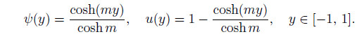
The variations of the amplitude of the normalized volume flow rate Q with m and k1 are presented in Fig. 4. From Fig. 4(a),it is observed that,when m increases,the amplitude of the volume flow rate Q increases and approaches a constant value for the given frequency Ω and the micropolar parameter k1. In order to verify the validity of Fig. 4(a),let us consider the limit situation where ω = χ = 0. In other words,we first consider the steady electroosmotic flow of the Newtonian fluid between two micro-parallel plates. Then,the nondimensional electrical potential and the velocity distribution can be reduced to
 |
|
Fig. 4 Dependence of amplitude of normalized volume flow rate on |
Therefore,the dimensionless volume flow rate becomes
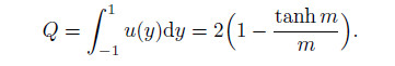
Since tanh m ≈ 1 when m > > 1,the volume flow rate Q will approach a constant (here Q → 2) when m is large (see Fig. 4(a)). If the working fluid is a micropolar fluid instead of a Newtonian fluid,the micropolar parameter k1 will affect the constant value that the volume flow rate Q approaches,but it will not change this trend.
Figure 4(b) shows that,when k1 increases from 0 to 1,the volume flow rate Q will finally decrease to zero for different values of the frequency Ω . This agrees well with the limiting case (iii) in Section 3. Figure 4(b) also clearly shows that,the amplitude of Q decreases when the frequency Ω increases. This is attributed to the effect of the parameter Ω on the amplitude of the velocity in Fig. 2.
4.3 Distribution of microrotationFigure 5 illustrates the variations of the dimensionless complex amplitude of the microrotation φ for different values of m and Ω . The amplitude of φ decreases when the frequency Ω increases. When Ω is low,smaller the value of m is,larger the amplitude of φ is. However,when Ω is large,a converse trend can be found. In addition,the oscillating characteristic becomes distinct when Ω increases. The reason is attributed to the fact that,when the frequency Ω is low,the velocity has almost no change in the bulk fluid region for larger m (see Fig. 2(a)),leading to the microrotation being mainly concentrated within the EDL region for larger m (see Fig. 5(a)). When the frequency is moderate (e.g.,Ω= 2.51),the fluctuation of the velocity gradually intensifies across the microchannel,and the microrotation strengths gradually from two solid walls to the channel center for larger m (see Fig. 5(b)).
 |
|
Fig. 5 Dimensionless microrotation distributions for different |
However,with the increase in the frequency Ω ,the velocity becomes flat in the channel center (see Fig. 2(d)). Therefore,the amplitudes of the microrotation become smaller and smaller,and finally approach zero away from the two EDLs of the walls for larger Ω (see Figs. 5(c) and 5(d)). The effects of the parameters m and Ω on the microrotation will be further discussed in the following content by introducing the concept of the microrotation strength. The effects of the parameter β on the microrotation are similar to the case of the velocity,and here we omit the discussion. For the sake of simplicity,the value of the parameter β will be fixed to be 1 in the following discussion.
4.4 Microrotation strengthIn order to study the effects of the relevant dimensionless parameters on the microrotation of the micropolar fluids,we introduce the concept of the dimensionless microrotation strength per unit area. Specifically,define

where

and the parameter β is fixed to be 1.
In Fig. 6,the amplitude of the microrotation strength W,defined above,is plotted for different k1 and Ω . There is obviously nonmonotonic dependence of W on k1 and Ω . When k1 → 0 or k1 → 1,the amplitude of W tends to zero (see Fig. 6(a)). This is attributed to the effect of the parameter k1 on the microrotation being shown in the limiting cases (ii) and (iii) in Section 3. This phenomenon can be explained further by introducing a characteristic penetration depth of the microrotation. Similar to the characteristic penetration depth of the velocity[28],we define the characteristic penetration depth σm of the microrotation as follows:

 |
|
Fig. 6 Amplitude of dimensionless microrotation strength |
When χ = 0,i.e.,k1 = 0,we have σm = 0. This means that the microrotation strength W is zero. When χ increases from zero,the penetration depth σm increases. Since the micropolar parameter k1 is a monotonically increasing function of χ for a fixed value of the dynamic viscosity μ,the amplitude of the microrotation strength will increase with the increase in k1 at the beginning. However,in addition to the penetration depth,the microrotation strength also depends on the amplitude of the microrotation by definition. Therefore,when χ >> μ,i.e.,k1 → 1,σm is greater than the characteristic length H. At this time,the energy dissipation caused by the viscosity coefficient χ will be dominated. Therefore,the amplitudes of the velocity and the microrotation turn out to be small. This finally leads to a decrease in the microrotation strength when k1 is near 1 (see Fig. 6(a)).
From Fig. 6(b),we can find that,when the value of Ω is low,e.g.,Ω < 1,the amplitude of W is almost a constant for the fixed parameters m and k1,and a smaller value of m gives a larger value of the amplitude of W. There are peaks for the amplitudes of W at moderate for large m. From Fig. 6(b),we may also observe that for the case of very high frequencies,the diffusion time scale is much greater than the oscillation time period. Therefore,there is no sufficient time for the flow angular momentum to diffuse far into the bulk region from the EDLs of the walls,and the penetration depth σm is small. Thus,the amplitude of W decreases to zero finally.
4.5 Stress tensorThe components σ21 and σ12 of the dimensionless stress tensor at the walls are odd functions of y by virtue of Eqs. (31),(34),and (37) and β = 1.
The amplitudes of σ21 at the wall y = −1 are presented in Fig. 7 for different values of m,k1,and Ω . It can be seen that when the frequency is small,e.g.,Ω < 1,the value of the micropolar parameter k1 does not affect the amplitude of the wall shear stress σ21,and |σ21| ≈ m. When Ω increases,there is a critical value Ω0 0 of the dimensionless frequency,which depends on the micropolar parameter k1 (see Fig. 7(b)). When Ω > Ω 0,the amplitude of the wall shear stress σ21decreases when Ω increases.
 |
|
Fig. 7 Variations of amplitude of dimensionless stress tensor σ21 at walls for different |
Unlike the wall shear stress σ21 ,the amplitude of σ12 depends on the micropolar parameter k1 at the low frequency Ω (see Fig. 8). When k1 → 1,the amplitude of σ12 tends to zero linearly for different m.
 |
|
Fig. 8 Variations of amplitude of σ12 at walls for different |
The behavior of the time periodic EOF of an incompressible micropolar fluid between two infinitely extended parallel-plates is investigated. The analytical solutions of the velocity and microrotation are derived under the Debye-H¨uckel linear approximation. The computational results show that the effects of the dimensionless electrokinetic width m and the frequency Ω on the velocity are similar to the case of the Newtonian fluid for a fixed micropolar parameter k1. The values of k1 show a significant monotonic effect on the velocity and the volume flow rate,i.e.,the amplitudes of the velocity and the volume flow rate will drop to zero when k1 increases from 0 to 1.
However,the factors affecting the microrotation are complex. The dependence of the microrotation on the micropolar parameter k1 and the frequency Ω is normally non-monotonic. When the value of k1 is small,the amplitude of the microrotation strength W increases with the increase in k1. However,the microrotation strength W begins to decrease when k1 is near 1. In the same way,there are peaks for the amplitudes of W at moderate values of for large m.
In addition,there is a critical value Ω0 0 of the dimensionless frequency. When Ω<Ω0 < 0,the value of the micropolar parameter k1 does not affect the amplitude of the wall shear stress σ21,and |σ21| ≈ m. However,when Ω> Ω 0,the amplitude of the wall shear stress σ21 will drop when Ω increases. For different values of the parameter m,the amplitude of σ12 tends to zero linearly when k1 → 1.
| [1] | Karniadakis, G., Beskok, A., and Aluru, N. Microflows and Nanoflows: Fundamentals and Simulation, Springer, New York (2005) |
| [2] | Laser, D. J. and Santiago, J. G. A review of micropumps. Journal of Micromechanics and Microengineering, 14, R35-R64 (2004) |
| [3] | Stone, H. A., Stroock, A. D., and Ajdari, A. Engineering flows in small devices: microfluidics toward a lab-on-a-chip. Annual Review of Fluid Mechanics, 36, 381-411 (2004) |
| [4] | Abhari, F., Jaafar, H., and Yunus, N. A. M. A comprehensive study of micropumps technologies. International Journal of Electrochemical Science, 7, 9765-9780 (2012) |
| [5] | Burgreen, D. and Nakache, F. R. Electrokinetic flow in ultrafine capillary slits. Journal of Physical Chemistry, 68, 1084-1091 (1964) |
| [6] | Xie, Z. and Jian, Y. Rotating electroosmotic flow of power-law fluids at high zeta potential. Colloids and Surfaces, A: Physicochemical and Engineering Aspects, 461, 231-239 (2014) |
| [7] | Jian, Y. J., Su, J., Chang, L., Liu, Q. S., and He, G. H. Transient electroosmotic flow of general Maxwell fluids through a slit microchannel. Zeitschrift für Angewandte Mathematik und Physik, 65, 435-447 (2014) |
| [8] | Jang, J. and Lee, S. S. Theoretical and experimental study ofMHD micropump. Sensors Actuators, A: Physical, 80, 84-89 (2000) |
| [9] | Pamme, N. Magnetism and microfluidics. Lab on a Chip, 6, 24-38 (2006) |
| [10] | Buren, M., Jian, Y., and Chang, L. Electromagnetohydrodynamic flow through a microparallel channel with corrugated walls. Journal of Physics, D: Applied Physics, 47, 425501 (2014) |
| [11] | Buren, M. and Jian, Y. Electromagnetohydrodynamic (EMHD) flow between two transversely wavy microparallel plates. Electrophoresis, 36, 1539-1548 (2015) |
| [12] | Dutta, P. and Beskok, A. Analytical solution of time periodic electroosmotic flows: analogies to Stokes' second problem. Analytical Chemistry, 73, 5097-5102 (2001) |
| [13] | Keh, H. J. and Tseng, H. C. Transient electrokinetic flow in fine capillaries. Journal of Colloid and Interface Science, 242, 450-495 (2001) |
| [14] | Kang, Y., Yang, C., and Huang, X. Dynamic aspects of electroosmotic flow in a cylindrical microcapillary. International Journal of Engineering Science, 40, 2203-2221 (2002) |
| [15] | Wang, X. M., Chen, B., and Wu, J. K. A semianalytical solution of periodical electro-osmosis in a rectangular microchannel. Physics of Fluids, 19, 127101 (2007) |
| [16] | Chakraborty, S. and Ray, S. Mass flow-rate control through time periodic electro-osmotic flows in circular microchannels. Physics of Fluids, 20, 083602 (2008) |
| [17] | Chakraborty, S. and Srivastava, A. K. A generalized model for time periodic electroosmotic flows with overlapping electrical double layers. Langmuir, 23, 12421 (2007) |
| [18] | Jian, Y., Yang, L., and Liu, Q. Time periodic electro-osmotic flow through a microannulus. Physics of Fluids, 22, 042001 (2010) |
| [19] | Jian, Y., Liu, Q., and Yang, L. AC electroosmotic flow of generalized Maxwell fluids in a rectangular microchannel. Journal of Non-Newtonian Fluid Mechanics, 166, 1304-1314 (2011) |
| [20] | Liu, Q., Jian, Y., and Yang, L. Time periodic electroosmotic flow of the generalized Maxwell fluids between two micro-parallel plates. Journal of Non-Newtonian Fluid Mechanics, 166, 478486 (2011) |
| [21] | Liu, Q., Jian, Y., and Yang, L. Alternating current electroosmotic flow of the Jeffreys fluids through a slit microchannel. Physics of Fluids, 23, 102001 (2011) |
| [22] | Bhattacharyya, A., Masliyah, J. H., and Yang, J. Oscillating laminar electrokinetic flow in infinitely extended circular microchannels. Journal of Colloid and Interface Science, 261, 12-20 (2003) |
| [23] | Chang, C. C. and Wang, C. Y. Starting electroosmotic flow in an annulus and in a rectangular channel. Electrophoresis, 29, 2970-2979 (2008) |
| [24] | Islam, N. and Wu, J. Microfluidic transport by AC electroosmosis. Journal of Physics: Conference Series, 34, 356-361 (2006) |
| [25] | Erickson, D. and Li, D. Analysis of alternating current electroosmotic flows in a rectangular microchannel. Langmuir, 19, 5421-5430 (2003) |
| [26] | Yang, J., Bhattacharyya, A., Masliyah, J. H., and Kwok, D. Y. Oscillating laminar electrokinetic flow in infinitely extended rectangular microchannels. Journal of Colloid and Interface Science, 261, 21-31 (2003) |
| [27] | Marcos, Yang, C., Ooi, K. T., Wong, T. N., and Masliyah, J. H. Frequency-dependent laminar electroosmotic flow in a closed-end rectangular microchannel. Journal of Colloid and Interface Science, 275, 679-698 (2004) |
| [28] | Minor, M., van der Linde, A. J., van Leeuwen, H. P., and Lyklema, J. Dynamic aspects of electrophoresis and electroosmosis: a new fast method for measuring particle mobilities. Journal of Colloid and Interface Science, 189, 370-375 (1997) |
| [29] | Oddy, M. H., Santiago, J. G., and Mikkelsen, J. C. Electrokinetic instability micromixing. Analytical Chemistry, 73, 5822-5832 (2001) |
| [30] | Das, S. and Chakraborty, S. Transverse electrodes for improved DNA hybridization in microchannels. AIChE Journal, 53, 1086-1099 (2007) |
| [31] | Das, S., Subramanian, K., and Chakraborty, S. Analytical investigations on the effects of substrate kinetics on macromolecular transport and hybridization through microfluidic channels. Colloids and Surfaces, B: Biointerfaces, 58, 203-217 (2007) |
| [32] | Eringen, A. C. Simple microfluids. International Journal of Engineering Science, 2, 205-217 (1964) |
| [33] | Eringen, A. C. Theory of micropolar fluids. Journal of Applied Mathematics and Mechanics, 16, 1-18 (1965) |
| [34] | Eringen, A. C. Microcontinuum Field Theories, II: Fluent Media, Springer, New York (2001) |
| [35] | Hayakawa, H. Slow viscous flows in micropolar fluids. Physical Review E, 61, 5477-5492 (2000) |
| [36] | Papautsky, I., Brazzle, J., Ameel, T., and Frazier, A. B. Laminar fluid behavior in microchannels using micropolar fluid theory. Sensors and Actuators, A: Physical, 73, 101-108 (1999) |
| [37] | Magyari, E., Pop, I., and Valkó, P. P. Stokes' first problem for micropolar fluids. Fluid Dynamics Research, 42, 025503 (2010) |
| [38] | Ariman, T., Turk, M. A., and Sylvester, N. D. Microcontinuum fluid mechanicsreview. International Journal of Engineering Science, 11, 905-930 (1973) |
| [39] | Ariman, T., Turk, M. A., and Sylvester, N. D. Application of microcontinum fluid mechanics. International Journal of Engineering Science, 12, 273-293 (1974) |
| [40] | Stokes, V. K. Theories of Fluids with Microstructures, Springer, New York (1984) |
| [41] | Lukaszewicz, G. Micropolar Fluids: Theory and Application, Birkhäuser, Basel (1999) |
| [42] | Siddiqui, A. A. and Lakhtakia, A. Steady electroosmotic flow of a micropolar fluid in a microchannel. Proceedings of the Royal Society, A: Mathematical, Physical and Engineering Sciences, 465, 501-522 (2009) |
| [43] | Siddiqui, A. A. and Lakhtakia, A. Debye-Hückel solution for steady electro-osmotic flow of micropolar fluid in cylindrical microcapillary. Applied Mathematics and Mechanics (English Edition), 34(11), 1305-1326 (2013) DOI 10.1007/s10483-013-1747-6 |
| [44] | Siddiqui, A. A. and Lakhtakia, A. Non-steady electro-osmotic flow of a micropolar fluid in a microchannel. Journal of Physics, A: Mathematical and Theoretical, 42, 355501 (2009) |
| [45] | Misra, J. C., Chandra, S., Shit, G. C., and Kundu, P. K. Electroosmotic oscillatory flow of micropolar fluid in microchannels: application to dynamics of blood flow in microfluidic devices. Applied Mathematics and Mechanics (English Edition), 35(6), 749-766 (2014) DOI 10.1007/s10483-014-1827-6 |
| [46] | Hunter, J. Zeta Potential in Colloid Science, Academic Press, New York (1981) |
| [47] | Ahmadi, G. Self-similar solution of imcompressible micropolar boundary layer flow over a semiinfinite plate. International Journal of Engineering Science, 14, 639-646 (1976) |
| [48] | Rees, D. A. S. and Bassom, A. P. The Blasius boundary-layer flow of a micropolar fluid. International Journal of Engineering Science, 34, 113-124 (1996) |
| [49] | Green, N. G., Ramos, A., Gonzalez, A., Morgan, H., and Castellanos, A. Fluid flow induced by nonuniform AC electric fields in electrolytes on microelectrodes, I: experimental measurements. Physical Review E, 61, 4011-4018 (2000) |