 2016, Vol. 37
Shanghai University
Article Information
- Hong QIN, Ming DONG
- Boundary-layer disturbances subjected to free-stream turbulence and simulation on bypass transition
- Applied Mathematics and Mechanics (English Edition), 2016, 37(8): 967-986.
- http://dx.doi.org/10.1007/s10483-016-2111-8
Article History
- Received Dec. 19, 2015
- Revised Mar. 17, 2016


2. Tianjin Key Laboratory of Modern Engineering Mechanics, Tianjin 300072, China
Laminar-turbulent transition in boundary-layer flows is a classical subject and has been studied for decades due to its practical importance. If the environmental disturbances are low in intensity,say less than 0.1% of the oncoming main-stream velocity,transition will follow a so-called natural route. In this process,Tollmien-Schlichting (T-S) waves are generated by the free-stream turbulence (FST) through some receptivity mechanism,and amplified exponentially as it convects downstream,leading to the breakdown of the laminar flow[1]. These instability modes are described by the discrete modes of Orr-Sommerfeld (O-S) and Squire equations in the linear stability theory[2]. In the presence of high-level FST (usually larger than 1%),Morkovin[3] described another transition route in which the amplification of the T-S waves is bypassed throughout the whole process,and it is referred to as bypass transition. Low-frequency perturbations with large amplitudes are generated within the boundary layer,which manifest themselves as elongated structures of the low and high speed fluid,as experimentally observed by Klebanoff [4]. These streaky structures grow algebraically until some saturated locations,after which they undergo long-period viscous decays. However,before streaks disappear,highfrequency disturbances grow rapidly due to the secondary instability mechanism[5],leading to the occurrence of turbulence at relatively low Reynolds numbers.
The formation of the streaks as a response to the FST is the first stage of bypass transition,and one mathematical approach to describe this scenario is based on the so-called unsteady boundary-region equations. By assuming that either the turbulent Reynolds number or the downstream distance (or both) is sufficiently small,Leib et al.[6] used the linearized boundaryregion equations to derive the Klebanoff-type disturbance in the boundary layer. Since the linearized analysis is not valid when the amplitudes of the external disturbances are relatively large,Ricco et al.[7] and Zhang et al.[8] used the nonlinear boundary-region equations to obtain streaks subjected to a pair of free-stream vortical disturbance (FSVD) and randomly-distributed FSVDs,respectively. It was found that FSVDs with low frequencies (usually ω = O(Re- Λ1),where ReΛ is the Reynolds number based on the spanwise length scale of the streaks Λ) seem to penetrate the boundary layer in the vicinity of the leading edge of the plate under the strong non-parallelism and generate streaky disturbances with the large amplitude of the streamwise velocity. The evolution of the streaky disturbances obtained numerically agreed well with experimental observations by Klebanoff [4],Matsubara and Alfredsson[9],and others,i.e.,after a dominantly algebraic growth,the streaks exhibit a long period of viscous attenuation. The secondary instability of the streaks was also analyzed by Ricco et al.[7] and Zhang et al.[8]. By choosing the streaks and the secondary modes of the latter work as the initial condition,Dong and Zhou[10] further carried out the direct numerical simulation (DNS) of the bypass transition and summarized the mechanism of the breakdown process. The boundary-region equation is essentially an initial value problem,i.e.,the patterns of streaks contain cumulated history effects.
Moreover,if the frequency of FSVD is relatively high,namely,ω » O(Re-1) (where Re is the Reynolds number based on the characteristic thickness of the boundary layer,and the boundary-layer thickness is of the same order as Λ),the process of the entrainment of FSVDs will be ‘local’,in which the boundary-layer response depends less on the information of the upstream flow. In this sense,a streaky profile can also be generated locally by an FSVD with the frequency O(Re-1) « ω « O(1),as shown by Dong and Wu[11]. Since Re increases with the streamwise coordinate x,the local receptivity mechanism,for a given low frequency,would operate at a relatively larger streamwise location.
The local entrainment mechanism is indeed attractive in terms of the numerical sense,i.e.,the inflow perturbations of the DNS can be solved only based on the local steady base flow. At first sight,the most natural mathematical model to describe the local receptivity process seems to be the continuous-spectrum solutions of the O-S and Squire equations,because their phase speed is approximately equal to that of FSVD. Jacobs and Durbin[12] firstly used this model to explain the phenomenon that free-stream vortices are expelled from the sheared region of the boundary layer,which was referred to as ‘shear sheltering’. Thereafter,Jacobs and Durbin[13] proposed a method to construct the turbulent inflow condition by using the continuous modes,and performed the DNS of bypass transition based on this inflow. Subsequently,a series of works using this method were carried out,such as Zaki and Durbin[14],Durbin and Wu[15],Zaki and Saha[16],and Brandt et al.[17]. Almost all the physical phenomena as observed experimentally in bypass transition also appeared qualitatively in these researches,i.e.,the evolution of the streaks,the rapid growth of high-frequency disturbances due to the secondary instability,and the emergence of turbulent spots. However,the inflow model itself consists of some contradictions with the physical phenomena.
As pointed out by Dong and Wu[11],the continuous modes exhibit two main non-physical aspects. First,any continuous mode simultaneously consists of two Fourier components with ei(k1x-ik2y+k3z-ωt) and ei(k1x+ik2y+k3z-ωt) (where k1,k2,and k3 denote the wavenumbers in the streamwise x-,wall-normal y-,and spanwise z-directions,respectively) in the external stream,whose amplitudes are interdependent. This is referred to as the ‘entanglement of Fourier components’. Second,for low-frequency disturbances,the solution exhibits a so-called ‘abnormal anisotropy’ behaviour,in which the amplitude of the streamwise velocity in the external stream is much larger than that of the transversal velocities. Both behaviours imply that the FSVDs cannot be chosen freely,but are determined by the presence of the boundary layer,which however conflicts with the physical fact,i.e.,all properties of FSVDs should be determined by the upstream condition,but unaffected by the boundary layer underneath. The causes of them are found to be directly related to the neglect of the non-parallel-flow effect,which actually play an equally important role as the convection terms in the linearized NavierStokes (N-S) equations. Dong and Wu[11] then proposed a large-Reynolds-number asymptotic approach,in which the non-parallelism is taken into account. The non-physical behaviours do not arise at all in the solution,and for Re-1 « ω « 1,a large oscillation of the streamwise velocity is observed at the outer reach of the boundary layer. Such disturbances represent a longitudinal streak. This solution is recently extended to the entrainment of short wavelength FSVDs and that in compressible boundary layers by Wu and Dong[18].
Therefore,the edge-layer solution could provide a rational way to impose the inflow perturbation for bypass-transition simulations subjected to the FST. However,this has not yet been proved numerically. The main task of this paper is to address this issue. Two remarks however need to be made. First,the edge-layer solution is based on the large-Reynolds-number asymptotic expansion,therefore,an error of O(1/Re) exists for the finite-Reynolds-number simulation. Second,the governing equation which Dong and Wu[11] used is deduced from the linearized N-S equation,and an error of O(Єu 2) (where Єu is the amplitude of the streamwise velocity,usually of the order O(0.1) for a streaky profile) is also present. Nevertheless,the errors do not bring any non-physical property,and are quantitatively predictable. Additionally,the nonlinear correction can be considered as it approaches downstream under the full N-S solver,which is also to be verified in this paper.
2 Physical problem 2.1 Physical modelThe physical model to be studied is an incompressible boundary layer past a three-dimensional semi-infinite flat plate,as shown in Fig. 1. The flow is described by a Cartesian coordinate system X = (x,y,z),where x,y,and z denote the coordinates in the streamwise,wall-normal,and spanwise directions,respectively. The reference length for normalization is chosen to be a characteristic boundary-layer thickness 

|
| Fig. 1 Sketch of physical model, where δ99 represents nominal thickness of boundary layer |
|
|

The Reynolds number Re is defined as
2.2 Steady basic flow
The steady solution of the boundary layer is the Blasius similarity solution. By introducing a slowly-varying coordinate 

where F is a function of η = y/

and the boundary conditions
2.3 Entrainment of FSVT
The edge-layer solution,as proposed by Dong and Wu[11],is used to describe the boundarylayer perturbation as a response to the FSVD.
The dispersion relation of the FSVD is

where the frequency ω,the wall-normal and spanwise wavenumbers γ and β are both real and given for spatial mode,while α = αr + iαi is complex with the real (αr) and imaginary (αi) parts representing the streamwise wavenumber and growth rate,respectively.
In the external stream,an FSVD is represented by

where 
The corresponding perturbation in the boundary layer can be expressed as a linear traveling wave,i.e.,

where 

If the FST is high in intensity,longitudinal streaks would be generated in the boundary layer. For an FSVD with the frequency of Re-1 « ωs « 1,wavenumbers of αs = O(ω) and (γs,βs) = O(1),and an amplitude of Єs = O(0.01),the generated streaky profile is expressed as
2.5 Entrainment of high-frequency disturbances
The longitudinal streaks (8) in boundary layer flows could not break down themselves. However,they can cause the secondary instability so that high-frequency disturbances would be excited and increase with large growth rates,leading to the occurrence of bypass transition. Thus,a certain number of high-frequency disturbances entrained by the FSVDs with small amplitudes should be introduced at the entrance of the computational domain for the simulation of bypass transition. The disturbances can be written as a summation of a series of Fourier modes,i.e.,

where N is the number of modes,and each Fourier mode can be expressed as
 (10)
(10) where the frequency of the entrained vortical disturbance ωn h = O(1),the wavenumbers (αh,n γh n,βh n) = O(1),and the amplitudes Єh n « O(0.01).
3 Numerical method 3.1 Governing equationThe DNS is based on the three-dimensional compressible N-S solver,which was used in Refs. [10, 19-21]. Since we are focusing on the incompressible case,we set the Mach number to be 0.2. The governing equations are written in the conservative form,
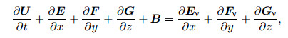 (11)
(11) where U is the conservative flux,

Equation (11) is discretized into a chosen cubic domain xl × yl × zl,and each grid point is denoted by (xi,yj,zk) with i ∈ [0,I],j ∈ [0,J],and k ∈ [0,K]. Uniform grids are used in both the streamwise and spanwise directions,while non-uniform grids clustered in the near-wall region are used in the wall-normal direction. The method to generate the wall-normal grids is introduced in Appendix B.
The nonlinear terms are discretized by employing the fifth-order finite-difference scheme with flux splitting according to positive and negative eigenvalues of the Jacobian matrix,while the viscous terms are discretized by employing the sixth-order central-difference scheme. The second-order Runge-Kutta (R-K) method is used for the time evolution. All the schemes can be found in Appendix C.
3.3 Boundary conditionsAt the entrance of the computational domain X0 = (x0,y,z),the flow field is composed of a steady base flow (3) and some certain unsteady disturbances. In principle,the Fourier spectrum of the disturbances in the external stream is continuous in the frequency,which however is not possible (and also not necessary) to be directly converted to the inflow perturbations in the numerical process. Therefore,we only select disturbances at typical frequencies as the inflow perturbations for the bypass-transition simulation,i.e.,a low-frequency disturbances (8) representing longitudinal streaks and a series of high-frequency disturbances (9). The inflow boundary condition is expressed as
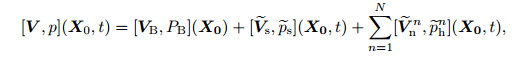 (12)
(12) where all the variables are introduced in Section 2.
A sponge region consisting of 40 points in the streamwise direction is imposed at the outlet of the computational domain,so that the disturbances can propagate further downstream without any reflection. No-slip and non-penetration conditions are employed at the wall. A characteristic non-reflecting boundary condition is employed at the upper boundary,i.e.,for the waves traveling outward,the boundary values are interpolated by the internal flow field,while for the waves traveling inward,the boundary values are imposed as the free-stream vortical disturbances. The periodic boundary condition is used in the spanwise direction.
Since our code is compressible,we also need to specify the boundary conditions for the temperature and density. Because the Mach number is low,the temperature and density would almost be uniform. Thus,their values at the boundary are fixed to be unit.
4 Evolution of single disturbance in boundary layers subjected to FSVDIn order to verify our inflow condition,we first study the evolution of a single disturbance as given by the edge-layer solution. In the simulation,the entrance of the computational domain is chosen to be 800δ r from the leading edge,at which the corresponding Reynolds number is Re = 800.
4.1 Evolution of low-frequency disturbance with small amplitudeThe parameters of the low-frequency disturbance introduced as the inflow perturbation are shown in Table 1,and its disturbance profiles are shown in Fig. 2,where all the quantities are normalized by the amplitude of the wall-normal velocity in the external stream. In the free stream,the magnitude of each velocity component has the same order,but the u-component is significantly enlarged at the edge of the boundary layer,which corresponds to the longitudinal streaks. The amplitude is sufficiently small so that its evolution can be treated as linearity.


|
Fig. 2 Disturbance profiles of  |
|
|
The computational domain is chosen as xl × yl × zl = 720×20.8×4.65,while the numbers of grid points are
Nx × N y × Nz = 1024 × 180 × 32.
Denote the instantaneous perturbation of the streamwise velocity as
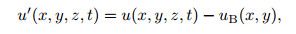 (13)
(13) where u is the instantaneous streamwise velocity. Figure 3 displays the streamwise evolution of u' obtained by our simulation at different wall-normal locations. It is clear that all curves are sinusoidally oscillatory along the streamwise direction with the amplitudes decaying. Meanwhile,the overall evolution of the instantaneous streamwise velocity can be predicted by the asymptotic solution (7) accurately,except that at the outer edge of the boundary layer,i.e.,y = 6.5 (see Fig. 3(b)),in which a slight phase lag is observed.

|
| Fig. 3 Evolution of instantaneous disturbance velocity u' (solid lines) in comparison with that predicted by asymptotic solution (dashed lines), where z = 0 and t = 11T with T = 227 representing period of disturbance |
|
|
Since the edge-layer solution is based on a large-Re asymptotic expansion,while the simulation is based on the finite Re,the disagreement of the two curves in Fig. 3(b),although tiny,is understandable. In order to confirm this,Fig. 4 further compares the wall-normal profile of u' as obtained by the numerical simulation with that by the asymptotic solution at a downstream location x = 400. For the low-Re case (Re = 800),the agreement between the two curves is quite good,except that at the outer edge of the boundary layer,i.e.,5 < y < 8. However,the error in this region is reduced dramatically if the Reynolds number is increased five times (Re = 4 000),implying that the simulated results approach the asymptotic solution as Re increases.

|
| Fig. 4 Wall-normal profiles of instantaneous disturbance velocity u' (solid lines) in comparison with that predicted by edge-layer solution (dashed lines), where z = 0, t = 11T , and x = 400 |
|
|
In bypass transition,longitudinal streaks are always generated by the relatively high FST. Therefore,in this section we take the amplitude of the FSVD to be Є = 0.03,and all other parameters are the same as displayed in Table 1.
In Fig. 5(a),the evolution of the instantaneous perturbation u' at the peak location of the edge-layer solution y = 4.6 is displayed. Being different from the linear case,the oscillation of u' is not exactly sinusoidal due to the nonlinear effect,and the time-averaged value deviates from zero appreciably. The mean-flow distortion of the streamwise velocity is defined as

|
| Fig. 5 Evolution of disturbances subjected to finite-amplitude and low-frequency FSVD at y = 4.6, z = 0, and t = 13T |
|
|
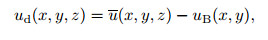 (14)
(14) where u is the time-averaged streamwise velocity. Figure 5(b) shows the evolution of the meanflow distortion ud at the same wall-normal position as in Fig. 5(a). In the region near the entrance,the mean flow is varying rapidly,because the introduced disturbance is obtained under the linear hypothesis. The nonlinear N-S solver allows the perturbations,as well as the mean-flow distortion,to swift adjust to the nonlinear solution. After about x = 160,the meanflow distortion becomes relatively smooth,and the nonlinear solution,representing physical streaks,is achieved.
Figure 6 further plots the instantaneous contours of the streamwise velocity u in the xy-plane at z = 0 and t = 13T ,and obvious low- and high-speed streaks near the edge of the boundary layer are observed.

|
| Fig. 6 Contours of instantaneous streamwise velocity in xy-plane, where z = 0 and t = 13T (thick solid lines: high-speed streaks (u > 1); dashed lines: low-speed streaks (u < 1); thin lines: u = 1) |
|
|
High-frequency FSVDs also play an important role in the bypass transition process since they generate the secondary-instability modes with high growth rates.
Table 2 shows the parameters of the high-frequency disturbance introduced as the inflow perturbation,where the amplitude is sufficiently small in order to keep the disturbances evolving linearly. The computational domain and the number of grid points are xl × yl × zl = 200 × 20.8 × 6.98 and N x × Ny × Nz = 312 × 180 × 32,respectively.
Figure 7 plots the disturbance profiles of the edge-layer solution subjected to a highfrequency FSVD. It is seen that the disturbance in the boundary layer is quite small.


|
Fig. 7 Disturbance profiles of  |
|
|
Figure 8 compares the instantaneous perturbation u' from the present simulation with that from the asymptotic solution (7). The curves agree precisely for each wall-normal position. It is found that the prediction made by the asymptotic theory for the high-frequency case is more accurate than that for the low-frequency case (see Fig. 3).

|
| Fig. 8 Evolution of instantaneous disturbance velocity u' (solid lines) in comparison with that predicted by asymptotic solution (dashed lines), where z = 0 and t = 11T with T = 22.7 |
|
|
In Fig. 9,we further compare the profiles of u' obtained by the two approaches,for two different Reynolds numbers. The agreement between the two curves is further improved if the Reynolds number is enlarged five times.

|
| Fig. 9 Wall-normal profiles of instantaneous disturbance velocity u' (solid lines) in comparison with that predicted by edge-layer solution (dashed lines), where z = 0, t = 11T , and x = 128 |
|
|
The DNS is performed in a cubic domain of 630×20.8× 13.96,and the number of grid points is 1 536×180× 192. The Reynolds number at the inlet boundary is also chosen to be 800.
The inflow perturbations,as given by (12),consist of a low-frequency streaky disturbance and a series of high-frequency disturbances. Table 3 displays the parameters of all the disturbances. Here,we artificially select 7 high-frequency disturbances,whose frequencies (ωh 1,ωh 2,· · · ,ω7 h) are 4,6,8,10,14,18,and 20 times of the low frequency ωs,so that the simulation has a period of 2π/ωs. The basic spanwise wavenumber is chosen to be β0 = 0.45,and the spanwise wavenumbers for the low-frequency βs and high-frequency (βh 1,βh 2,· · · ,βh 7) disturbances are 3 and 2 times of β0,respectively. The wall-normal wavenumbers γs and (γh 1,γh 2,· · · ,γh 7) for all disturbances are chosen to be the same for simplicity. Since the spectra of the free-stream disturbances as observed experimentally exhibit large amplitudes for low-frequency components and small amplitudes for high-frequency components,we simply assume that the low-frequency disturbance introduced has an amplitude of Єs = 0.03,and high-frequency disturbances have amplitudes of 0.001.

The coefficients of the skin friction based on either the spanwise- and time-averaged velocity u or instantaneous velocity u are defined as
 (15)
(15) where subscript ‘w’ denotes the quantities at the wall.
The streamwise distributions of Cf and Cf are shown in Fig. 10. Both curves remain almost constant for x < 230,which agrees with the skin-friction curve obtained from the Blasius profile (see the dotted line). After x ≈ 230,the mean skin-friction curve Cf undergoes a dramatic rise,implying the breakdown of the laminar flow. After peaking at about x = 360,the Cf curve declines gradually,roughly in agreement with the empirical curve of the turbulent boundary layer[22]. Meanwhile,the instantaneous skin-friction curve Cf experiences similar overall trend,but exhibits extremely large fluctuations,especially in the region near x = 300. The sharp drop at this location appears as a turbulent-laminar interface,representing a relaminarization phenomenon during the transition process.

|
| Fig. 10 Streamwise distributions of instantaneous (Cf, solid line, with t = 8T and z = 8) and timeaveraged (Cf, dashed line) skin frictions, where dotted and dot-dashed lines are reference curves for laminar and turbulent boundary lays, respectively |
|
|
Figure 11 plots the contours of the streamwise disturbance velocity u' within the transitional region,i.e.,200 < x < 400. The time scale T = 227 is the period of the introduced lowfrequency disturbance,and t/T denotes different phase. It is clear from each sub-figure that three streaks exist in the laminar region,and evolve with oblique nature until their breakdown after x = 300,corresponding to the sharp increase of the Cf or Cf curve,as shown in Fig. 10. The following chaotic fluctuations near x = 400 indicate that the turbulent stage has been reached. Additionally,at the instant of t/T = 0,a turbulent spot appears at about x = 220 and z = 8. After a period of 0.125T ,the spot convects to the position where x ≈ 240,and two more turbulent spots appear on the other two streaks. Then,they convect further downstream and merge with the strong fluctuation in the turbulent stage at t/T = 0.375. After that,new turbulent spots appear at the early laminar stage again and are expected to experience the same scenario.

|
| Fig. 11 Contours of streamwise disturbance velocity at five different instants, where y = 2.5 or y ≈ 0.49δ99 |
|
|
The disturbance velocity u' can be decomposed into the Fourier series,
 (16)
(16) where ω0 = 0.027 66 is the fundamental frequency,β0 = 0.45 is the fundamental spanwise wave number,and m and n denote the orders of the harmonic components. For instance,
In Fig. 12,the streamwise evolution of the Fourier components 


|
Fig. 12 Streamwise distribution of amplitude of Fourier components  |
|
|
Figure 13 compares the profiles of the low-frequency component 

|
Fig. 13 Low-frequency disturbance  |
|
|

|
Fig. 15 Profiles of Fourier components   |
|
|
Figure 14 further compares the mean-flow distortions 

|
Fig. 14 Mean-flow distortion  |
|
|
The profiles of four typical high-frequency Fourier components for different x are shown in Fig. 15. Primarily,the high-frequency FSVDs seem to be expelled from the boundary layer (see Figs. 15(a) and 15(b)). However,the presence of streaks encourages them to entrain the boundary layer and formulate secondary modes (see Figs. 15(c) and 15(d)). The latter have peak values relatively far from the wall,e.g. at about y = 2,which are supported by the secondary instability of the streaky profile,and by no means related to viscous T-S waves whose eigenfunctions are plotted in Fig. 15(f). These disturbances are amplified 10 times in such a short interval 200 < x < 300,which corresponds to less than a half of the wavelength of the streaks (about 230). The turbulent stage has already been reached at x = 400,where all the disturbances are almost of the same order of magnitude.
In turbulent boundary layers,the mean-velocity profile and the wall-normal coordinate are often measured by wall units,i.e.,
 (17)
(17) where 

|
| Fig. 16 Mean velocity profiles at x = 500 and x = 600 |
|
|
In this paper,the asymptotic solution based on the ‘edge-layer’ equation,which was proposed by Dong and Wu[11],is verified to be a proper mathematical model to represent the boundarylayer response to the FSVD numerically. It is found that if the FSVD is sufficiently small in the amplitude,its downstream evolution can be predicted by the asymptotic solution accurately,although there exists an small error caused by the finite-Re effect. However,the latter can be reduced if the simulation is performed under larger Reynolds numbers. If the FSVD has a finite amplitude with a low frequency,longitudinal streaks within the boundary layers can be obtained after a certain distance downstream of the entrance of the computational domain due to the nonlinear correction in the direct simulation.
The DNS of the boundary-layer bypass transition is performed by introducing a series of ‘edge-layer’ solutions as the inflow perturbations. In the early laminar stage,only the lowfrequency FSVD has a high penetration depth,while the high-frequency FSVDs are expelled from the boundary layer. The low-frequency disturbance in the boundary layer,appearing as streaks,is the dominant perturbation for quite a long distance until its breakdown. Meanwhile,the low-frequency disturbance distorts the mean flow,leading to the generation and rapid amplification of high-frequency disturbances due to the secondary instability mechanism. Since the streaks oscillate in the low frequency,the secondary modes increase intermittently,leading to the relaminarization (appearing as a turbulent-laminar interface) phenomenon during the transition process. In the turbulent stage,the amplitudes of all the disturbances tend to the same order of magnitude,and the mean profiles satisfy the classical log law of turbulent boundary layers. It is confirmed that the ‘edge-layer’ asymptotic solution can be used as a proper inflow perturbation in the simulation of bypass transition subjected to the high FST.
Appendix AThe flow field is represented by the vector
 (A1)
(A1) where ρ, u, v, w denote the density, streamwise, wall-normal, and spanwise velocities, respectively, and es = p/(ρ(γ − 1)) + q2 represents the total energy, in which p is the pressure, γ = 1.4 is the ratio of the specify heats, and q2 = u2 + v2 + w2 /2 is the kinetic energy.
 (A2a)
(A2a)  (A2b)
(A2b)  (A2c)
(A2c) where hs = q2 + pγ/(ρ(γ − 1)).
 (A3a)
(A3a)  (A3b)
(A3b)  (A3c)
(A3c) where

with T being the temperature, μ and k the dynamical viscosity and heat conductivity, respectively.
 (A4)
(A4) where UB denotes the Blasius solution.
Appendix BThe grid distance in the wall-normal direction is stretched according to
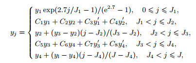 (B1)
(B1) where y1, y2, y3, y4 represent the wall-normal coordinates at the connecting points, which divide the domain into five zones, J1, J2, J3, J4 represent the ordinal number of the connecting points, and y1', y2 ',y3',y4'are the derivative of y on j at these points. C1, C2, C3, C4, C5, C6, C7, and C8 are polynomial coefficients of Hermite interpolation formula, which are expressed as
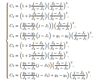 (B2)
(B2) In this paper, (y1, y2, y3, y4) and (J1, J2, J3, J4) are chosen to be (0.3, 1.8, 7.3, 9.0) and (10, 40, 120, 135),respectively, and the distribution of wall-normal grids is shown in Fig. 17.
Appendix CA typical nonlinear term 
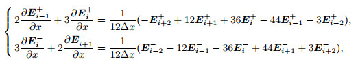 (C1)
(C1) where E+i and Ei− are Steger and Warming’s positive and negative fluxes[23], respectively, and Δx is the grid space in the streamwise direction.
A typical viscous term 
 (C2)
(C2) The second-order R-K method used in time advancing can be expressed as
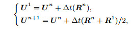 (C3)
(C3) where Δt is the time step, R1 = 

| [1] | Kachanov, Y. S. Physical mechanisms of laminar-boundary-layer transition. Annual Review of Fluid Mechanics, 26(1), 411-482 (1994) |
| [2] | Schmid, P. J., & Henningson, D. S. Stability and Transition in Shear Flows. Springer, New York (2001) |
| [3] | Morkovin, M. V. On the Many Faces of Transition. Springer, New York, 1-31 (1969) |
| [4] | Klebanoff, P. S. Effect of free-stream turbulence on a laminar boundary layer. Bulletin of the American Physical Society, 16(11), 1323-1334 (1971) |
| [5] | Andersson, P., Brandt, L., Bottaro, A., & Henningson, D. S. On the breakdown of boundary layer streaks. Journal of Fluid Mechanics, 428, 29-60 (2001) |
| [6] | Leib, S. J., Wundrow, D. W., & Goldstein, M. E. Effect of free-stream turbulence and other vortical disturbances on a laminar boundary layer. Journal of Fluid Mechanics, 380, 169-203 (1999) |
| [7] | Ricco, P., Luo, J., & Wu, X. Evolution and instability of unsteady nonlinear streaks generated by free-stream vortical disturbances. Journal of Fluid Mechanics, 677, 1-38 (2011) |
| [8] | Zhang, Y., Zaki, T., Sherwin, S., and Wu, X. Nonlinear response of a laminar boundary layer to isotropic and spanwise localized free-stream turbulence. The 6th AIAA Theoretical Fluid Mechanics Conference, American Institute of Aeronautics and Astronautics, Reno (2011) |
| [9] | Matsubara, M., & Alfredsson, P. H. Disturbance growth in boundary layers subjected to freestream turbulence. Journal of Fluid Mechanics, 430, 149-168 (2001) |
| [10] | Dong, M., & Zhou, H. A simulation on bypass transition and its key mechanism. Science China Physics, 4, Mechanics and Astronomy, 56(4), 775-784 (2013) |
| [11] | Dong, M., & Wu, X. On continuous spectra of the Orr-Sommerfeld/Squire equations and entrainment of free-stream vortical disturbances. Journal of Fluid Mechanics, 732, 616-659 (2013) |
| [12] | Jacobs, R. G., & Durbin, P. A. Shear sheltering and the continuous spectrum of the OrrSommerfeld equation. Journal of Fluid Mechanics, 10, 2006-2011 (1998) |
| [13] | Jacobs, R. G., & Durbin, P. A. Simulations of bypass transition. Journal of Fluid Mechanics, 428, 185-212 (2001) |
| [14] | Zaki, T. A., & Durbin, P. A. Mode interaction and the bypass route to transition. Journal of Fluid Mechanics, 531, 85-111 (2005) |
| [15] | Durbin, P., & Wu, X. Transition beneath vortical disturbances. Annual Review of Fluid Mechanics, 39(1), 107-128 (2007) |
| [16] | Zaki, T. A., & Saha, S. On shear sheltering and the structure of vortical modes in single- and two-fluid boundary layers. Journal of Fluid Mechanics, 626, 111-147 (2009) |
| [17] | Brandt, L., Schlatter, P., & Henningson, D. S. Transition in boundary layers subject to freestream turbulence. Journal of Fluid Mechanics, 517, 167-198 (2004) |
| [18] | Wu, X., & Dong, M. Entrainment of short-wavelength free-stream vortical disturbances in compressible and incompressible boundary layers. Journal of Fluid Mechanics, 797, 683-728 (2016) |
| [19] | Dong, M., Zhang, Y., & Zhou, H. A new method for computing lamina-turbulent transition and turbulence in compressible boundary layers-PSE+DNS. Applied Mathematics and Mechanics (English Edition), 29(12), 1527-1534 doi:10.1007/s0483-008-1201-z (2008) |
| [20] | Dong, M., & Zhou, H. The improvement of turbulence modeling for the aerothermal computation of hypersonic turbulent boundary layers. Science China Physics, 2, Mechanics and Astronomy, 53(2), 369-379 (2010) |
| [21] | Dong, M., & Zhou, H. The effect of high temperature induced variation of specific heat on the hypersonic turbulent boundary layer and its computation. Science China Physics, 11, Mechanics and Astronomy, 53(11), 2103-2112 (2010) |
| [22] | White, F. M., & Corfield, I. New York. McGraw-Hill Education, Viscous Fluid Flow, 1-425 (2006) |
| [23] | Steger, J. L., & Warming, R. F. Flux vector splitting of the inviscid gasdynamic equations with application to finite-difference methods. Journal of Computational Physics, 40(2), 263-293 (1981) |