 2016, Vol. 37
Shanghai University
Article Information
- Jianxin LIU, Shaolong ZHANG, Song FU
- Linear spatial instability analysis in 3D boundary layers using plane-marching 3D-LPSE
- Applied Mathematics and Mechanics (English Edition), 2016, 37(8): 1013-1030.
- http://dx.doi.org/10.1007/s10483-016-2114-8
Article History
- Received Oct. 20, 2015
- Revised Mar. 14, 2016


2. School of Aerospace Engineering, Tsinghua University, Beijing 100181, China


How to compute the growth rate accurately and robustly is crucially important in the eN method for predicting the location of the transition onset in boundary layers correctly. It is obvious that the boundary layer in practice is often three dimensional (3D). To obtain an accurate amplified rate is thus often difficult. A conventional methodology for searching the spatial amplified rates of the disturbances is a linear stability theory (LST). The dispersion relations of the disturbances q(y) = 


An alternative choice for the spatial growth-rates of the disturbances in boundary layers is a linear parabolic stability equation (LPSE). If the stationary base flow equation is subtracted from the unsteady flow equation,stability equations can be derived. The stability equation can be used to describe the linear and nonlinear evolution of the disturbances. However,the governing equations are elliptic. It means that we have to solve the equations in the whole spatial region. In order to bypass the elliptic difficulty,Herbert[3] parabolized the governing equations by dropping the streamwise derivatives in viscous terms. These parabolized equations are called parabolized stability equations (PSE). This method offers an efficient marching solution along the streamwise direction to obtain the instability characteristics in boundary layers. Owing to not neglecting the streamwise variations of the base flows and the instability modes in the convection terms,the non-parallel effect is also accounted for in the PSE. With ignoring the nonlinear terms in the PSE,the LPSE can be derived to describe the linear evolution of a disturbance. Unlike the LST solving the EVP at a local location,the LPSE procedure only solves a linear equation system at one location to obtain the growth of the disturbances directly. It makes solution procedure more robust.
Previously,the PSE procedure was widely adopted to solve the instability problems in 2D and quasi-2D boundary layers with ignoring the spanwise variation of the base flow. It is successful to predict the linear and nonlinear development of the disturbances in 2D boundary layers. Bertolotti et al.[4] investigated the linear and nonlinear instability in an incompressible boundary layer by the PSE. Chang and Malik[5] calculated the linear and nonlinear development of the disturbances in the compressible Blasius boundary layers at Ma = 1.6 using the compressible PSE. On the research of the instability in the Gö ortler flow and crossflow vortices,the PSE was also selected to obtain the satisfied results of the vortices[6-7]. Chang et al.[8] extended the PSE with real gas effects to study the reacting flows in hypersonic boundary layers in 1997.
However,lots of the boundary layers are 3D. Then,a 3D-PSE approach,a 3D extension of the 2D-PSE,is developed accounting for the spanwise non-parallel effect of the base flow. There are three procedures to implement the 3D-PSE,the plane-marching procedure,the surfacemarching one,and the line-marching one. The surface-marching approach was advised firstly by Herbert[9]. This marching solution is able to be performed along any direction on the body surface. This concept is quite similar to the numerical procedure of the 3D boundary layer equations. The line-marching approach means that the PSE marching is performed locally along a pre-identified line path (e.g. streamline or group velocity line) on the surface. The surface-marching and line-marching approaches solve the PSE without crossing plane solutions in the yz-plane,called the “local” PSE approaches. They have good efficiency in the PSE solutions. And the two “local” approaches were implemented in the LASTRAC.3d,a code developed by Chang[10] in NASA Langley for the stability and transition analysis. However,more assumptions were adopted in these local procedures. When 
The plane-marching LPSE procedure for the 3D boundary layer suitable for the full Mach number region is developed in the present work. And this implement is to be the cross-validation by the 2D-LPSE,LST,bi-global EVP,and direct numerical simulation (DNS),not only for a global problem but also for a local one.
2 Governing equations and numerical algorithms 2.1 Bi-global EVP equationsWe donate x as the streamwise direction,y the wall-normal direction and z the spanwise direction. Consider the 3D linear disturbances equations in a compressible boundary layer below (normalized by the boundary layer thickness at the inlet and the far-field flow),i.e.,

Here,φ = [ρ,u,v,w,T]T are density,velocities and temperature disturbances in the flow,and the coefficient matrices Γ,A,B,C,etc. in the above equations are the functions of all three coordinates for 3D boundary layers. Γ,A,B,C,D are the inviscid coefficient matrices,and Vij (i = 1,2,3; j = 1,2,3) are the viscous ones. Detailed expressions of these matrices can be found in Ref. [19]. Equation (1) is an elliptic form which requires a significant amount of computational resource to be solved.
Similar to the ones in 2D boundary layers,with a quasi-parallel assumption along the streamwise direction,the disturbance φ can be expressed as

Here,

The matrices on the left side of the above equation are

Here,a 2D-EVP is formed with the shape-function 
Accounting for the non-parallel effect of the boundary layers,the streamwise variations of the shape-functions and the streamwise wavenumbers of the disturbances are all considered. The disturbance can be expressed as

Here,

Here,we have

Generally,the frequency of the disturbance is known,while the shape functions and the streamwise wavenumber are unknown in the 3D-LPSE. Equation (6) can be solved by a plane-marching procedure. Though a reasonably large scale linear algebraic equations system is required to be solved,this procedure is more robust and easier than solving the EVP. Compared with Eq. (3) for the bi-global EVP,the streamwise gradients of the shape functions are accounted for as the first terms in the left hand of the 3D-LPSE (see Eq. (6)). Therefore,the streamwise non-parallel effect of the boundary layers can be described well in the 3D-LPSE.
In fact,the 3D-LPSE increases the efficiency of the solution process by simplification of the linear disturbance equations which describe the linear evolution of the disturbances in boundary layers. On the one hand,Eq. (1) is simplified into a parabolic form. The equations can be easily solved by a marching process along the streamwise direction. On the other hand,in the LPSE,the fast scale part of the instability is resolved into two slow scale parts: the shape function and the phase function. The variations of these functions in the streamwise direction are the order of O(1/Re). It means that the disturbances can be captured by a far coarser grid compared with solving Eq. (1).
The 2D-PSE is only “near parabolic” due to the streamwise pressure gradient term. Li and Malik[21] researched the numerical characteristics of this problem and gave the approach to reduce the elliptic characteristics of the streamwise pressure gradient term in the PSE. In the 3D-LPSE,this problem remains. Following Li and Malik’s work[21] in the 2D-PSE,the streamwise gradient of the pressure shape function is neglected. The streamwise disturbances pressure gradients are treated as

An ambiguity still exists in the PSE formulation. A normalization condition is required in order to close the problem in the PSE. Considering the shape function and the phase function varying slowly in the streamwise direction,the auxiliary equation is adopted in the present work following the normalization condition used in the 2D-PSE,i.e.,

Here,Ω is the whole domain of the cross plane yz-plane. This normalization implies that the kinetic energies of the shape functions are identical along the streamwise direction. The complex streamwise wavenumber α here is only the function of x in the Eqs. (5) and (9). It means that the growth rate and the streamwise wavenumber of the instability mode in one cross plane (yz-plane) are constant,i.e.,a spatial “bi-global” instability problem at one streamwise location.This instability problem can be seen as a secondary instability problem in streamwise vortices in shear flows. However,the constant α becomes inadequate when a local instability problem is carried out. Chang[10] advised α as a function of x and z to describe the disturbances mode variation in the spanwise direction,though no work has been performed. Here,α is the local wavenumber. At present,this advice is adopted for a local instability problem. Equation (9) is only adopted for a bi-global instability problem. An alternative normalization is used below for the local problem in the 3D-LPSE,i.e.,
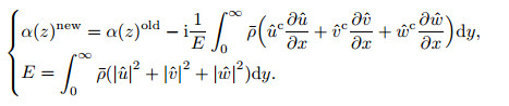 (10)
(10) For alleviating the numerical error,if E is small enough,the streamwise wavenumber α is to be set as the neighbor value.
The streamwise wavenumber α here is not the “true” physical value. In a spatial problem,the nonparallel boundary layer is growing in the streamwise direction. It makes the shape functions vary in this direction. Then,the physical growth rates and wavenumbers depend on the flow quantity and location inside the boundary layers. This is very different from the local procedure (2D-EVP). In the local procedure,the growth rates are independent of that for the parallel flow assumption. It means that the shape functions have no variation in the streamwise direction. However,there are the variations of the shape functions in a realistic boundary layer. When a disturbance is travelling in the streamwise direction,not only the amplitude is increasing or damping,but also the shape functions have a 1/Re order of the variations. Therefore,the instability of the flow must be predicted by the PSE accounting for the variation of the disturbance qualities.
In the PSE,the effective streamwise wavenumber can be evaluated as follows:
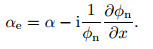 (11)
(11) Here,φn is a normalized disturbance quantity. One can use the integral quantity such as the disturbance kinetic energy to define the “averaged” non-parallel value.
Actually,the PSE solution is just one kind of the stability equations. It means that it can give the spatial evolution of the disturbances directly,and the effective growth rate here is just a description for evaluating the dynamics of the flow. Then,Eq. (5) is adopted if comparing the evaluated evolution with the DNS results.
Dirichlet boundary conditions are used at the isothermal wall and the free-stream,
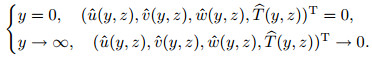 (12)
(12) If the wall is adiabatic,the temperature boundary condition at the wall is
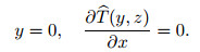 (13)
(13) Furthermore,the continuity equations at the wall and the free stream can be used as the auxiliary conditions. The spanwise boundary conditions rely on cases. In our cases,periodic boundary conditions are adopted.
The PSE requires an initial condition to start the streamwise marching procedure. Here,the eigenfunctions obtained from the O-S equations are adopted to initiate marching. The initial guess value of the complex streamwise wavenumber is also obtained from the O-S equations. In other words,the initial conditions are obtained by the bi-global EVP for the 3D-LPSE.This initial approach would make a “transient” region near the inlet boundary in the PSE because the non-parallel effect is neglected in the O-S equations. However,the PSE approach will alleviate this phenomenon for considering the non-parallel effect downstream.
2.3 Spatial discretizationGenerally,the first-order implicit backward Euler scheme is adopted in the streamwise direction. And higher orders of accuracy numerical discretization schemes are necessary in both spanwise and wall-normal directions. Both spectral methods and high-order finite-difference methods were reported in the spatial discretization[17]. The spectral methods offer the higher accuracy numerical discretization and less requirement of the storage. However,periodic boundary conditions are necessary. The high-order finite-difference methods are easy to be used when gird point distributions are non-uniform. At present,the fourth-order central finite-difference scheme is adopted in the wall-normal and spanwise directions (see Ref. [19]). It is easy to be used to consider the complexity for the boundary conditions in the spanwise direction.
The number of wall-normal grid points is over 250,with over one half of points inside the boundary layer region. In the spanwise direction,the dimension and the distribution of the grid points are dependent on the problem. Generally,there are about 100 grid points in the spanwise direction when solving a 3D problem.
2.4 Solution process of 3D-LPSEWith the spatial discretization,the 3D-LPSE (see Eq. (6)) can be rewritten in a simple form of
 (14)
(14) Here,L0 and L1 are the complex linear operator matrices with the given streamwise wavenumber at the i + 1 streamwise location. The rank of the square complex matrix is 5NyNz for the 3D-LPSE instead of 10N yNz for the 2D-EVP. It means that the PSE is much easier to solve.
The 3D-LPSE formulations are solved with the iterative procedure in the following manner:
(i) Start with an initial guess of the complex streamwise wavenumber α0 i+1 = αi.
(ii) Solve Eq. (14) to obtain a new eigenfunction 
(iii) Update αn+1 i+1 with Eq. (9) for a global problem or Eq. (10) for a local problem.
(iv) Check if |αn+1 i+1 - αn i+1| < ε. If yes,the true eigenfunctions and streamwise wavenumber are obtained. If no,go back to the step (ii).
This procedure is implemented along the whole computation domain. The 3D-LPSE formulations are solved in the cross plane one by one along the streamwise direction. There is a very large-scale equations system for a cross-plane solution in Eq. (14),and the coefficient matrices are complex and unsymmetrical. Here,PARDISO is adopted to solve the large-scale linear equations[22]. It supports the parallelization with OpenMP and has a higher efficiency.
3 Validation and results 3.1 Comparison with 2D-LPSE results in Blasius boundary layersThe plane-marching 3D-LPSE approach is a 3D extension of the 2D-LPSE. The method is validated by the comparison with 2D-LPSE in a Blasius boundary layer.
A classical case is selected to compare with the 2D-LPSE. As validated in Ref. [15],the 3DLPSE approach is validated by the 2D-LPSE results for the linear instability in a hypersonic flat-plate boundary layer. The parameters are shown in Table 1.

The base flow is hypersonic in Case 1. There are often two unstable modes in the hypersonic cases,the first mode and the Mack mode. In a 2D hypersonic boundary layer flow,the least stable Mack mode is 2D,while the least stable Tollmien-Schlichting (T-S) mode is 3D. Here,Case 1 corresponds to the first mode which is often 3D. Figure 1 shows the real part and the imaginary part of the streamwise wavenumber α in Case 1. There is a transient variation at the inlet. However,the transient effect will be alleviated downstream. It can be seen that the result in the 3D-LPSE agrees perfectly with the one in the 2D-LPSE. The velocity and temperature eigenfunctions of the instability mode are shown in Fig. 2. The eigenfunctions of the 3D method also match perfectly with the 2D results.

|
| Fig. 1 Streamwise wavenumber (Case 1), (a) real part; (b) imaginary part |
|
|

|
| Fig. 2 Velocity and temperature eigenfunctions (Case 1), (a) velocity; (b) temperature |
|
|
The result indicates that the difference between the two methodologies is insignificant for the 2D boundary layers. In other words,the 3D-LPSE can be applied to describe the instability of the 2D flows,and the plane-marching 3D-LPSE approach is compatible with the 2D-LPSE. This conclusion is consistent with Ref. [15].
3.2 Linear evolution of spanwise wave-packet disturbances in boundary layersThe plane-marching 3D-LPSE approach also can be used to compute the “local” instability problem. In order to validate this methodology for the “local” instability in a boundary layer,the linear evolution of spanwise wave-packet disturbances in flat-plate boundary layers is selected. In these cases,the auxiliary condition to normalize the eigenfunction must be selected as Eq. (10). It implies that the disturbances may have different instability characteristics at every spanwise location. Therefore,the local “streamwise wavenumber” in the 3D-LPSE is different at different spanwise locations.
The spanwise wave-packet disturbances are introduced into an boundary layer at the inlet.The Gauss function is adopted to modulate the disturbances which are obtained from the O-S equations. The amplitude distribution of the disturbance can be expressed as
 (15)
(15) Here,A is the amplitude of the disturbance,zc is the location of the centerline in the spanwise direction,a is the parameter to control the spanwise Gauss distribution,and c.c. means conjugate complex. When a = 0,the disturbance is purely 2D at the inlet. Figure 3 shows a typical distribution of the disturbance at the inlet when a = 0.002. The base flow here is selected as the Blasius boundary layer. Both incompressible and compressible cases are investigated. The parameters are listed in Table 2.

|
| Fig. 3 Amplitude distribution at inlet (a = 0.002) |
|
|

|
Figure 4 shows the comparison of the results in Case 2 with the DNS at the spanwise centerline[23]. Before x = 200,the evolution of the disturbance predicted by the 3D-LPSE agrees excellently with the result of the DNS. After x = 200,the amplitude of disturbance in the DNS decreases at first and then increases quickly for the nonlinear effect. It suggests that the plane-marching 3D-LPSE can give an accurate prediction in the linear region,and it can be applied to investigate the linear evolution of the spanwise wave-packet disturbance in an incompressible boundary layer.

|
| Fig. 4 Development of wave-packet disturbance at z = 64 in incompressible flat-plate boundary layer |
|
|
In a hypersonic boundary layer,as in the incompressible boundary layer,the linear evolution obtained by the DNS also confirms the prediction obtained by the 3D-LPSE. Figure 5 shows the comparison among the results of the 3D-LPSE,the LST,and the DNS at three different spanwise locations. These three locations correspond to the different local amplitudes of the wave-packet disturbance at the inlet,respectively. It can be seen that the results of the 3DPSE are excellently consistent with the DNS while the LST underestimates the evolution of the wave-packet disturbance. Especially at the location off the centerline,it is obvious that the 3DLPSE is better than the LST. It suggests that the plane-marching 3D-LPSE approach can also be employed as the tool to predict the linear evolution of a spanwise wave-packet disturbance in a hypersonic boundary layer. Actually,as discussed above,the evolution of the disturbance is obtained directly by the 3D-LPSE. It may be the reason why the results of the 3D-LPSE are in more excellent agreement with the DNS than the local eigenvalue method.

|
| Fig. 5 Development of wave-packet disturbance in hypersonic flat-plate boundary layer, (a) z = 150; (b) z = 142.4; (c) z = 139.8 |
|
|
Due to the imbalance between the centrifugal force and the normal pressure gradient near a concave surface,it is known that the fluids behave as counter-rotating longitudinal vortices which are called Gö ortler vortices. It is a classical 3D boundary layer. Because of the large variation in the spanwise direction,the local analysis cannot be adopted to obtain the characteristic of the instability. Therefore,the bi-global procedures are developed to analyse the instability in such a 3D boundary layer instead of the local analysis. Generally,the linear secondary instability analysis is the one of these bi-global procedures. It can be used to investigate the bi-global instability of the Gö ortler vortices. Li and Malik[7] investigated the temporal instability of the incompressible Gö ortler vortices by the linear secondary instability analysis with the Floquet technique and gave the eigenfunction distributions. The linear secondary instability procedure is often to solve a 2D-EVP. At present,instead of the linear secondary instability analysis,the spatial bi-global instability will be investigated by solving Eq.(3). The solutions of this EVP can be used to validate the plane-marching 3D-LPSE approach which also can be adopted to investigate the spatial bi-global instability of the flows. In addition,the solution of the spatial 2D-EVP also provides an approximate initial condition to be introduced in the plane-marching 3D-LPSE procedure. In order to validate the plane-marching 3D-LPSE suitable for the full Mach number region,the results of the DNS in the hypersonic and incompressible cases are selected to be the benchmark.
The base flows are obtained by solving the parabolized partial differential equation (see Ref. [7]). All lengths,temperature,and the mean flow quantities are non-dimensionalized by the viscous length scale l0,the free-stream temperature T∞,and the free-stream velocity U∞,respectively. The length scale is defined by l0 = (νx0/U∞)1/2. Here,ν is the kinematic viscosity,and x0 is the location of a reference station. The Reynolds number is defined by Re = U∞l0/ν. The Gö ortler number G = Re/R1/2 is another important parameter. Here,R is the dimensionless curve radius.
Both incompressible and hypersonic cases are investigated in the present work. The parameters of the Gö ortler vortices are shown in Table 3. Here,the base flow in Case 4 is the incompressible flow,while the one in Case 5 is the hypersonic flow. Figure 6 shows the velocity contours of the Gö ortler flow. It is obvious that the streamwise variations of the flows are significant.


|
| Fig. 6 Velocity contours of Gö ortler flow, (a) incompressible; (b) hypersonic |
|
|
Figure 7 shows the contours of streamwise velocity and its gradient at X = 92 cm in Case 4. The velocity contours have a mushroom-like distribution. The velocity is relatively lower in the “peak” region and higher in the “valley” region. The boundary layer varies rapidly from the peak region to the valley one along the spanwise direction. There are significant 3D characteristics in the z-direction. As shown in Figs. 7(b) and 7(c),the velocity profiles have inflection points both in the normalwise direction and in the spanwise direction,which leads to invisid instabilities. There are often different unstable modes in the Gö ortler flows. According to the spanwise distribution characteristics of eigenfunctions,they can be divided into odd and even modes. The even mode is symmetric,while the odd one is antisymmetric. We only consider the least stable odd mode and even mode for their higher growth rates. The spatial bi-global instability of the Gö ortler vortices is investigated by Eq.(3). The frequency of the disturbances focused on is 190 Hz. Figure 8 plots the eigenfunctions contours at X = 92 cm. The even mode corresponds to the normalwise velocity gradient while the odd one corresponds to the spanwise velocity gradient. These contours are similar to the results in Ref.[7].

|
Fig. 7 Contours of streamwise velocity and its gradient at X = 92 cm in Case 4, (a) U with magnitudes 0 to 1; (b)   |
|
|

|
| Fig. 8 u eigenfunctions (absolute value) of spatial EVP at X = 92 cm, (a) even mode; (b) odd mode, where dash lines are velocity contours of base flow |
|
|
The same spatial bi-global instability problem can be studied using the 3D-LPSE. In the 2D-EVP,the parallel base flow and eigenfunction in the x-direction are assumed. However,the streamwise non-parallel effect is considered in the 3D-LPSE. In order to make a validation,an ideal Gö ortler flow is selected to be the base flow,and two different procedures are used to compute the linear spatial growth rate. This ideal Gö ortler flow is obtained by freezing the base flow in the cross plane yz-plane at X = 92 cm along the streamwise direction. It is obvious that the boundary layer has no variation in the steamwise direction,and the eigenfunctions at each streamwise location are the same because of the same profiles. It means that the difference between the 3D-LPSE and the 2D-EVP can be ignored in this streamwise 3D flow. The bi-global stability problem is preformed by both the 3D-LPSE and 2D-EVP. For the even mode,the growth rate obtained by the 3D-LPSE is about (0.468 5 cm),and this value agrees excellently with the one (0.468 9 cm) obtained by the 2D-EVP. For the odd mode,the growth rate is 0.393 6 cm by the 3D-LPSE,which matches perfectly with the value obtained by the 2D-EVP. It suggests that the plane-marching 3D-LPSE approach is identical to the 2D-EVP in an incompressible parallel boundary layer.
Actually,the realistic Gö ortler flow is the non-parallel 3D boundary layer (see Fig. 6(a)). The streamwise non-parallel effect makes the instability different between the 3D-LPSE and the 2D-EVP,because the streamwise non-parallel effect is ignored in the 2D-EVP. The even mode and the odd mode obtained by the 2D-EVP procedure are introduced into the flow at the inlet,respectively. The evolutions of the two different unstable modes are obtained by the plane-marching 3D-LPSE. Figure 9 shows the comparison of the streamwise distributions of the growth rates between the even mode and the odd mode obtained by the two different methodologies. There is a little difference between the 3D-LPSE and the 2D-EVP because of the streamwise non-parallel effect of the base flow. Figure 10 shows the comparison of the linear evolution obtained by the different methodologies. It can be seen that the result of the 3D-PSE agrees excellently with the DNS,while the 2D-EVP procedure overestimates the amplitude of the disturbance by about 200% at least when the instability is the even mode. For the odd mode,although the prediction of 2D-EVP is not too bad,the 3D-LPSE procedure is still a better choice for evaluating the linear evolution of the disturbance in the Gö ortler flows. It seems the growth rates obtained by the 3D-LPSE and the 2D-EVP are different. Nevertheless,the streamwise variation of the shape functions,which is considered in the 3DLPSE,has a significant contribution to the spatial instability. In summary,it suggests that the plane-marching 3D-LPSE can describe the linear spatial bi-global instability in the non-parallel incompressible flow well.

|
| Fig. 9 Spatial growth rates of unstable mode in imcompressible non-parallel Gö ortler flow, (a) even mode; (b) odd mode |
|
|

|
| Fig. 10 Comparison of linear evolution in realistic imcompressible Gö ortler flow, (a) even mode; (b) odd mode |
|
|
The plane-marching 3D-LPSE approach is also studied in the 3D hypersonic Gö ortler flow for the bi-global instability problem. Figure 11 shows the streamwise velocity and temperature contours at X = 2.4 m in the yz-plane in Case 5. It is obvious that the hypersonic Gö ortler vortices are very similar to the ones in the incompressible flow. In other word,the bi-global instability analysis ought to be used to obtain the unstable modes. In the present case,the disturbances with the frequency 50 kHz are focused on because they are often unstable in the base flow of Case 5. Different from the incompressible case,the least stable modes and the secondary one are both odd modes,and the amplified rates are much larger than the ones of the even mode. Therefore,only the least stable odd mode is concentrated on at present. Figure 12 shows the shape functions of the least stable odd mode in Case 5. The shape functions here are obtained by the local 2D-EVP. The eigenfunctions also correspond to the inflections of the base flow as the ones in Case 4.

|
| Fig. 11 Contours in yz-plane of velocity and temperature in Case 5 (X = 2.4 m), (a) velocity; (b) temperature |
|
|

|
| Fig. 12 Contours of eigenfunctions (absolute value) of spatial EVP at X = 2.4 m in Case 5, least stable odd mode, (a) density; (b) velocity; (c) temperature |
|
|
The validation process as the one in the incompressible case is performed in the hypersonic case. The 3D-LPSE approach is validated with the 2D-EVP in the artificial ideal 3D boundary layer. The ideal base flow is obtained by the same freezing methodology as the one in the incompressible case. Here,the base flow in the yz-plane at X = 2.4 m is selected to be freezed. The growth rate of the least stable odd mode of the flow obtained by the 3D-LPSE is about 0.333 cm. It is identical to the one (0.333 cm) obtained by the 2D-EVP method. The 3D-LPSE procedure is in a perfect agreement with the 2D-EVP in the hypersonic parallel boundary layer. It means that the 3D-LPSE is an equivalent tool for the instability in the 3D flow with no streamwise variation.
The result by the plane-marching 3D-LPSE also agrees excellently with the one by the 2DEVP in the realistic non-parallel boundary layer as in the incompressible case. As shown in Fig. 13,the spatial growth rate obtained by the 3D-LPSE is close to the one obtained by the 2D-EVP. The streamwise non-parallel effect is considered in the 3D-LPSE. Therefore,there is a little difference in the two approaches. The results are also validated by the DNS. Figure 14 shows the comparison of the linear evolution of the disturbance obtained by the DNS and the amplitude distribution predicted by the 3D-LPSE and the 2D-EVP. It can also be seen that there is still a significant divergence between the prediction of the 2D-EVP and the investigation of the DNS because no streamwise variation of the shape-function is considered in the 2DEVP,while the predicted curve by the 3D-LPSE agrees with the result of the DNS excellently. Conclusively,it verifies that the plane-marching 3D-LPSE approach supplies a satisfied choice to compute the spatial growth rate in the hypersonic 3D boundary layer.

|
| Fig. 13 Spatial growth rate of least stable mode in hypersonic non-parallel Gö ortler flow |
|
|

|
| Fig. 14 Comparison of linear evolution in realistic hypersonic Gö ortler flow |
|
|
The crossflow vortices are also classical 3D boundary layers in engineering. They are usually generated by the crossflow instability over the swept-wings. As the Gö ortler vortices,the spatial bi-global instability of the crossflow vortices can also be investigated by the traditional 2DEVP and the 3D-LPSE. Therefore,they are selected as the benchmark for validating the planemarching 3D-LPSE suitable for the full Mach number region.
In order to fill the gap of the high subsonic flow,the subsonic crossflow vortices are selected. The model is the NLF0415 airfoil with the swept angle of 45°. The parameters of the crossflow are listed in Table 4. The vortices are obtained by solving the Navier-Stokes equations,and Fig. 15 shows the contours of the flow. Here,x is the direction of vortex axis,and z is the transverse direction.

|
| Fig. 15 Velocity contours of crossflow vortices |
|
|

Figure 16 shows the contours of the x-velocity in the yz-plane at X = 370 mm. The contours of the flow are different from those of the Gö ortler vortices,i.e.,the flow is neither symmetric nor antisymmetric. However,the instability mechanism is similar. Then,the unstable modes corresponding to the normalwise inflection point are called “y-mode” while the ones corresponding to the transverse inflection point are called “z-mode”. In Case 6,the disturbances with the frequency 33 kHz are concerned. The least mode of the profile is z-mode which is plotted in Fig. 17. The eigenfunction here is obtained by the local 2D-EVP procedure,and the local spatial growth rate is about 0.138 mm. This value is also obtained by the 3D-LPSE procedure in the artificial ideal boundary layer which is uniform along the x-direction. It indicates that the 3D-LPSE approach is the same as the local 2D-EVP procedure if ignoring the variation of the flow in the x-direction.

|
| Fig. 16 Contours of x-velocity in yz-plane at X =370 mm in Case 6 |
|
|

|
| Fig. 17 Contours of x-velocity eigenfunction (absolute value) of spatial EVP at X = 370 mm in Case 6, least stable z-mode |
|
|
The spatial instabilities are also investigated in the realistic non-parallel crossflow vortices. As shown in Fig. 18,the growth rates obtained by the 3D-LPSE are about 10%-20% greater than the ones obtained by the 2D-EVP. Figure 19 shows the comparison of the development obtained by the 3D-LPSE,the 2D-EVP,and the DNS. It can be seen that the 3D-LPSE procedure predicts the linear development of disturbance excellently,while the 2D-EVP underestimates the evolution. It suggests that the 3D-LPSE procedure is a better choice for predicting the linear development of the disturbance in a high subsonic spatially developing 3D flow.

|
| Fig. 18 Spatial growth rate of least stable mode in non-parallel crossflow vortices |
|
|

|
| Fig. 19 Comparison of linear development in realistic crossflow vortices |
|
|
In this paper,the 3D-LPSE method suitable for the full Mach number region is developed for the three boundary layers by the plane-marching procedure,especially when the boundary layer varies significantly in the spanwise direction. In this method,the streamwise and spanwise nonparallel effects are both considered. The plane-marching procedure is more robust and efficient in the 3D boundary layers than the traditional 2D-EVP method. We verify this method in incompressible,subsonic,supersonic and hypersonic boundary layers,e.g.,Blasius boundary layers for a 2D instability,and Gö othler vortices and crossflow vortices for a 3D instability problem. The results obtained by the 2D-LPSE,the LST,the 2D-EVP,and the DNS are selected as the benchmark,respectively. We examine the compatibility of the 3D-LPSE firstly. Both local instability and global instability are also investigated. For the local instability problem,the linear development of the spanwise wave-packet disturbances is investigated in the incompressible and the hypersonic boundary layers. The evolution of the disturbances agrees excellently with the benchmark in the linear region. For the global instabilities problem,Gö ortler flows and crossflow vortices,the classical 3D boundary layers,are selected as the base flow. The linear instabilities are investigated in the incompressible and hypersonic Gö ortler vortices cases and the the subsonic crossflow vortices case. The results show the prediction obtained by the 3D-LPSE is in excellent agreement with the results of the DNS. It suggests that the plane-marching 3D-LPSE procedure is a more satisfied choice for the instability in a spatial developing 3D flow.
The plane-marching 3D-LPSE procedure extends the 2D-LPSE method for an instability problem to 3D boundary layers and provides an efficient,accurate,and robust tool to analyze these kinds of instabilities accounting for the non-parallel effect in the streamwise and the spanwise directions. Future works should focus on the better efficiency of this procedure. And it can be applied to the roughness induced transition problem in the hypersonic flows or other instability and transition problems in 3D boundary layers.
Acknowledgements Thanks to Jie REN in Tsinghua University for supplying the Gö othler flow,Xuezhi LU in Tianjin University for supplying the crossflow vortices,and Runjie SONG in Tianjin University for supplying the evolution on the wave-packet disturbance in the hypersonic boundary layer.| [1] | Saric, W. S., & Nayfeh, A. H. Nonparallel stability of boundary layer flows. Physics of Fluids, 18, 945-950 (1975) |
| [2] | El-Hady, N. M. Nonparallel instability of supersonic and hypersonic boundary layers. Physics of Fluids A:Fluid Dynamics, 3, 2164-2178 (1991) |
| [3] | Herbert, T. Parabolized stability equations. Annual Review of Fluid Mechanics, 29, 245-283 (1997) |
| [4] | Bertolotti, F. P., Herbert, T., & Spalart, P. R. Linear and nonlinear stability of the Blasius boundary layer. Journal of Fluid Mechanics, 242, 441-474 (1992) |
| [5] | Chang, C. L., & Malik, M. R. Oblique-mode breakdown and secondary instability in supersonic boundary layers. Journal of Fluid Mechanics, 273, 323-360 (1994) |
| [6] | Malik, M. R., Li, F., Choudhari, M. M., & Chang, C. L. Secondary instability of crossflow vortices and swept-wing boundary-layer transition. Journal of Fluid Mechanics, 399, 85-115 (1999) |
| [7] | Li, F., & Malik, M. R. Fundamental and subharmonic secondary instabilities of Görtler vortices. Journal of Fluid Mechanics, 297, 77-100 (1995) |
| [8] | Chang, C., Vinh, H., and Malik, M. Hypersonic boundary-layer stability with chemical reactions using PSE. The 28th AIAA Fluid Dynamics Conference, Snowmass Village (1997) |
| [9] | Herbert, T. On the stability of 3D boundary layers. The 28th AIAA Fluid Dynamics Conference, American lnstitute of Aeronautics and Astronautics, Snowmass Village (1997) |
| [10] | Chang, C. L. LASTRAC. 3d: transition prediction in 3D boundary layers. The 34th AIAA Fluid Dynamics Conference, American lnstitute of Aeronautics and Astronautics, Portland (2004) |
| [11] | Hall, P., & Horseman, N. J. The linear inviscid secondary instability of longitudinal vortex structures in boundary layers. Journal of Fluid Mechanics, 232, 357-375 (1991) |
| [12] | Högberg, M., & Henningson, D. Secondary instability of cross-flow vortices in Falkner-SkanCooke boundary layers. Journal of Fluid Mechanics, 368, 339-357 (1998) |
| [13] | Choudhari, M., Li, F., Wu, M., Chang, C. L., Edwards, J., Kegerise, M., and King, R. Laminarturbulent transition behind discrete roughness elements in a high-speed boundary layer. The 48th AIAA Aerospace Sciences Meeting Including the New Horizons Forum and Aerospace Exposition, American lnstitute of Aeronautics and Astronautics, Orlando (2010) |
| [14] | Choudhari, M., Li, F., and Edwards, J. E. Stability analysis of roughness array wake in a highspeed boundary layer. The 47th AIAA Aerospace Sciences Meeting Including the New Horizons Forum and Aerospace Exposition, American lnstitute of Aeronautics and Astronautics, Orlando (2009) |
| [15] | Hu, S. and Zhong, X. Nonparallel stability analysis of compressible boundary layer using 3-D PSE, The 37th AIAA Aerospace Sciences Meeting Including the New Horizons Forum and Aerospace Exposition, American lnstitute of Aeronautics and Astronautics, Reno (1999) |
| [16] | Broadhurst, M. S., & Sherwin, S. J. The parabolised stability equations for 3D-flows:implementation and numerical stability. Applied Numerical Mathematics, 58, 1017-1029 (2008) |
| [17] | Paredes, P., Theofilis, V., Rodriguez, D., and Tendero, J. A. The PSE-3D instability analysis methodology for flows depending strongly on two and weakly on the third spatial dimension. The 6th AIAA Theoretical Fluid Mechanics Conference, American lnstitute of Aeronautics and Astronautics, Honolulu (2011) |
| [18] | De, Tullio N., Paredes, P., Sandham, N. D., & Theofilis, V. Laminar-turbulent transition induced by a discrete roughness element in a supersonic boundary layer. Journal of Fluid Mechanics, 735, 613-646 (2013) |
| [19] | Zhang, Y., & Zhou, H. Verification of the parabolized stability equations for its application to compressible boundary layers. Applied Mathematics and Mechanics (English Edition), 28, 987-998 doi:10.1007/s10483-007-0801-3 (2007) |
| [20] | Lehoucq, R. B., Sorensen, D. C., and Yang, C. ARPACK Users' Guide: Solution of Large-Scale Eigenvalue Problems with Implicitly Restarted Arnoldi Methods, Society for Industrial and Applied Mathematics, Philadelphia (1998) |
| [21] | Li, F., & Malik, M. R. On the nature of PSE approximation. Theoretical and Computational Fluid Dynamics, 8, 253-273 (1996) |
| [22] | Schenk, O., & Gärtner, K. Solving unsymmetric sparse systems of linear equations with PARDISO. Future Generation Computer Systems, 20, 475-487 (2004) |
| [23] | Li, J. The Numerical Simulation of Transition for Spanwise Wavepacket Disturbances in Boundary Layers and the Prediction by the PSE Method (in Chinese), Ph. D. dissertation, Tianjin University (2012) |