 2016, Vol. 37
Shanghai University
Article Information
- Chao XU, Dongyang SHI, Xin LIAO
- Low order nonconforming mixed finite element method for nonstationary incompressible Navier-Stokes equations
- Applied Mathematics and Mechanics (English Edition), 2016, 37(8): 1095-1112.
- http://dx.doi.org/10.1007/s10483-016-2120-8
Article History
- Received Oct. 9, 2015
- Revised Mar. 14, 2016


2. School of Mathematics and Statistics, Zhengzhou University, Zhengzhou 450001, China
Let Ω in R2 be a bounded domain with a Lipschitz-continuous boundary ∂Ω. We consider the following two-dimensional nonstationary incompressible Navier-Stokes equations:


where u = (u1,u2) denotes the fluid velocity vector field,p is the pressure filed,f = (f1,f2) is the given vector field,and ν > 0 is the constant inverse Reynolds number.
It is well known that the nonstationary incompressible Navier-Stokes equations are one of the main equations studied in mathematical physics and fluid mechanics fields. Numerous works have been devoted to numerical solutions of the above equations using finite element methods (FEMs). For example,we quote Ref. [1] for the conforming FEM,Ref. [2] for the fully discrete penalty FEM,Ref. [3] for the variational multiscale method,and Refs. [4]-[6] for the different stabilized FEMs. Recently,the nonconforming elements,which are usually easier to be constructed to satisfy the inf-sup condition than the conforming ones,received more and more attention for (1)−(4). In Ref. [7],the finite difference streamline diffusion method about the nonconforming P1nc /P0 element pair of Ref. [8] was discussed with regard to a large Reynolds number. Shi and Wang[9] extended the above element pair to anisotropic meshes,and the error estimates for the velocity in the L2-norm and the broken H1-norm,as well as for the pressure in the L2-norm were obtained.
On the other hand,there have appeared some excellent studies on the superconvergent analysis of mixed nonconforming FEMs for the stationary Stokes and Navier-Stokes equations. For example,the L2 projection method was discussed for the Stokes problem[10-11]. The basic idea of L2 projection method is to construct a new finite element (FE) approximation in a finite-dimensional space corresponding to a coarse mesh,and the difference in the mesh sizes can be used to achieve a better convergent rate after the post-processing procedure. Later,this idea was extend to solve the nonlinear Navier-Stokes equations[12]. In Refs. [13] and [14],the integral identities techniques and interpolation postprocessing operators about the nonconforming CQ1rot /P0 element pair were applied to the Stokes equations and Stokes equations with damping,and obtained the superconvergent results,respectively.
In this paper,we will use CQ1rot /P0 element pair to solve the nonstationary problem (1)−(4) through different approaches from the application of the nonconforming P1nc /P0 element pair in Ref. [9],and we obtain the superclose and superconvergent results for the velocity u in the broken H1-norm and the pressure p in the L2-norm with reasonable regularity of the exact solution (u,p).
The rest of the paper is organized as follows. In Section 2,we briefly introduce the variational formulation for (1)-(4) and some preliminaries. In Section 3,we state the construction of the nonconforming mixed FE scheme about CQ1rot /P0 element pair. In Section 4,we present the corresponding error estimates. In Section 5,the proper post-processing technique is applied. In Section 6,a numerical experiment is carried out to confirm our theoretical results.
We will use the notations for the Sobolev spaces Wm,q(Ω) with the norm 

To introduce a variational formulation,set


where

It is well known that for u ∈ H01 (Ω) there hold

Here and later,C denotes a positive constant independent of the mesh parameter h and may be different at each occurrence.
Besides,for all u,v,w ∈ V ,the trilinear form b(· ; · ,·) satisfies the following properties[16]:


 (10)
(10) where

In order to guarantee the properties of the existence and uniqueness of the solution (u,p) about problems (1)-(4),the following further assumptions and lemma are needed:
(i) Assume that Ω is regular in the sense that the unique solution (u,p) ∈ (V ,M) of the stationary Stokes problem,i.e.,−Δu+ ∇p = g and ∇u = 0 in Ω,and u|∂Ω = 0 for a prescribed g ∈ Y exists and satisfies 
(ii) The initial velocity u0 ∈ D(A) and the body force f(x,t) ∈ L2(0,T ;Y ) are assumed to satisfy

Lemma 1[17] Assume that (i) and (ii) hold. Then,for a given T > 0 there exists a unique solution (u,p) satisfying

where ρ(t) =min{1,t}.
3 Construction of nonconforming mixed FE schemeLet Th be a rectangular partition of the convex polygon domain Ω. For a given element K ∈ Th with a center point (xK,yK),its four vertices are denoted by a1(x1,y1),a2(x2,y2),a3(x3,y3),a4(x4,y4) and four edges by 


Define the affine mapping FK : 

The Q1rot element space Rh is defined by[18-20]

where 
Then,the CQ1rot element space CRh is defined by[13, 21]

For the velocity,we choose Vh = CRh ×CRh as the approximation space. Furthermore,we define

which is a norm over Vh.
Let

be a piecewise constant FE space,and Mh ⊂ Qh is used to approximate the pressure,which consists of piecewise constants with respect to Th. The local basis functions for Mh on a 2 × 2 patch of T are indicated in Fig. 1,i.e.,

and the subdivision T2h is obtained by dividing each element of Th into four congruent rectangles.

|
| Fig. 1 Local basis functions of Mh |
|
|
The associated interpolation operators 

Then,for all u ∈ H2(Ω) ∩H01(Ω) or q ∈ H1(Ω) ∩ L02 (Ω),there hold
 (11)
(11)  (12)
(12) Lemma 2[14] Assume that u ∈ Hm+1(Ω) ∩H01 0 (Ω),we have
 (13)
(13)  (14)
(14) Lemma 3[13-14] For vh ∈ Vh,we have
 (15)
(15) Lemma 4 For vh ∈ Vh,we have
 (16)
(16) Proof The proof of first result of (16) is similar to Lemma 4.3 in Ref. [22]. Thus,we only give the proof of the second one. Let 
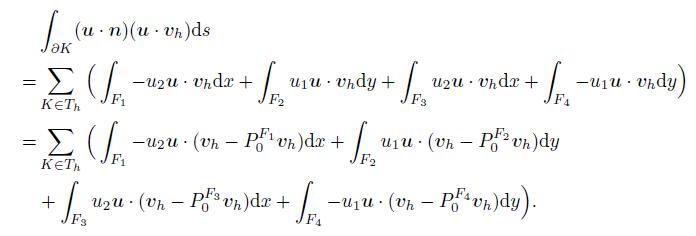 (17)
(17) Since 
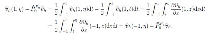 (18)
(18) Hence,for a given element K,there holds

A direct computation implies

which leads to
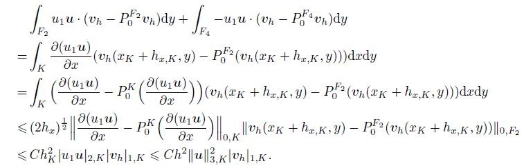 (19)
(19) Similarly,
 (20)
(20) The second desired result in (16) follows from (19) and (20). The proof is completed.
4 Convergence analysisThe nonconforming FE approximation of (5)-(7) is as follows: to find (uh,ph) ∈ Vh ×Mh such that
 (21)
(21)  (22)
(22)  (23)
(23) where

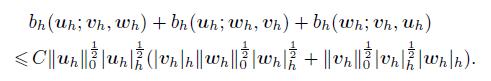
The above trilinear form bh(·; ·,·) satisfies the following properties[22]:
 (24)
(24) where

With the similar argument to Ref. [23],we have
 (25)
(25) which leads to

Therefore,
 (26)
(26) Using the Sobolev inequalities[24-25] and combining (25) with k = 1,we can derive
 (27)
(27) Furthermore,we have
 (28)
(28) It has been shown in Refs. [13] and [21] that the pair (Vh,Mh) satisfies the discrete inf-sup condition,i.e.,
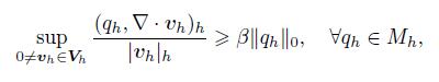 (29)
(29) where β is a positive constant independent of h.
Now,we introduce a subspace Zh of Vh as

In order to carry out the error estimates,we introduce the notations ρ = u − Πhu and θ = Πhu − uh,where θ ∈ Zh.
Lemma 5 Under the assumptions (i) and (ii) and 
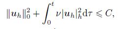 (30)
(30) 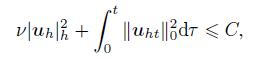 (31)
(31)  (32)
(32) Here and later,
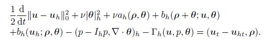
Proof Firstly,for any vh ∈ Zh,taking vh = 2uh in (21),there holds
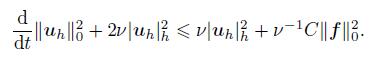 (33)
(33) Integrating the above inequality from 0 to t and noting

we obtain the result (30) by Lemma 1.
Secondly,combining (1) with (21),we find that
 (34)
(34) where
 (35)
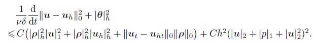
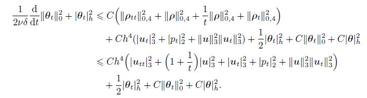
(35) Choosing vh = θ and rearranging terms in (34),we get
 (36)
(36) Using (26) and Lemmas 3 and 4,we have

and

Combining these inequalities with (34),and noting 
 (37)
(37) Then,by integrating (37) from 0 to t and noting that
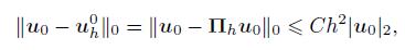 (38)
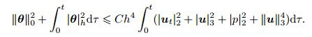
(38) it follows from Lemma 1 and (30) that
 (39)
(39) To estimate the term 
 (40)
(40) The terms bh(uh;u,uht) and (f,uht) can be bounded as follows:

Obviously,we have
 (41)
(41) Subsequently,combining the above estimates with (40),we get
 (42)
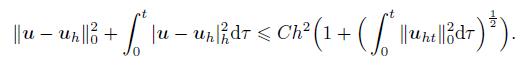
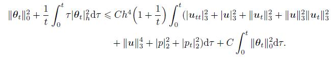
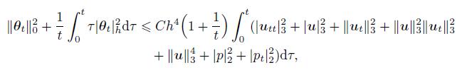
(42) Now,integrating (42) from 0 to t and using (39),we have
 (43)
(43) which implies
 (44)
(44) Combining (43)-(44) with (39) gives the desired results (31) and (32).
Lemma 6 Under the assumptions of Lemma 5,there hold
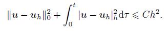
 (45)
(45)  (46)
(46) Proof By differentiating (21) with respect to the time t and noting vh ∈ Zh,it holds
 (47)
(47) Set vh = uht,we have
 (48)
(48) which implies
 (49)
(49) Using (28) and Young’s inequality,we have

which,combining with (49),gives
 (50)
(50) Integrating (50) and using Lemma 5,we obtain the result (45).
Taking vh = uhtt in (47),we find
 (51)
(51) which can be rewritten as
 (52)
(52) It follows from (41) that

and

Then,combining these estimates with (52),it follows from Lemma 5 that
 (53)
(53) Similarly,multiplying (53) by t,integrating from 0 to t,and using Lemma 5,we obtain that

i.e.,

he proof is completed.
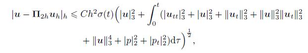
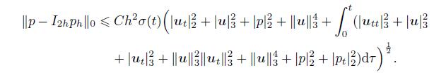
Theorem 1 Let (u,p) ∈ V ×M and (uh,ph) ∈ Vh ×Mh be the solutions of (1)-(4) and (21)-(23),respectively. Assume that u,ut,utt ∈ H3(Ω),p,pt ∈ H2(Ω),and ν−1
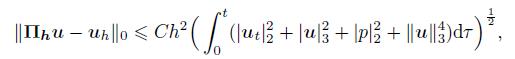 (54)
(54) 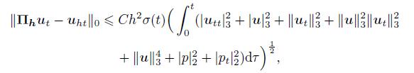 (55)
(55) 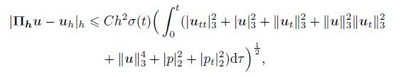 (56)
(56) where σ(t) = 
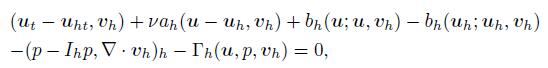
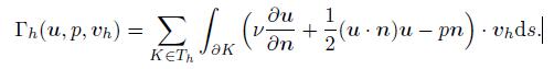
Proof From (1) and (21),we know
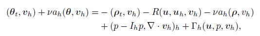 (57)
(57) where
 (58)
(58) Setting vh = θ in (57),we obtain
 (59)
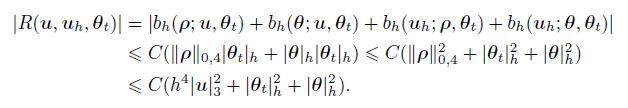
(59) Applying (24),Lemmas 2-5,and the results (3.11) and (3.13) in Ref. [13],we have
 (60)
(60) and
 (61)
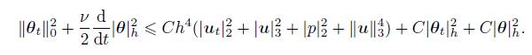
(61) Noting ν−1
 (62)
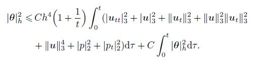
(62) Integrating (62) from 0 to t and noting θ(0) = 0,we obtain
 (63)
(63) By the Gronwall lemma,it holds
 (64)
(64) Then,(54) can be derived directly.
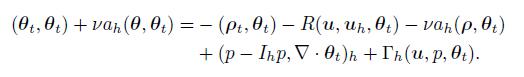
Secondly,we prove (55). Differentiating both sides of (57) with respect to t and setting vh = θt,we have
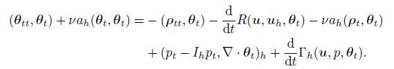 (65)
(65) By (24),(28),and Lemmas 2-5,we can obtain
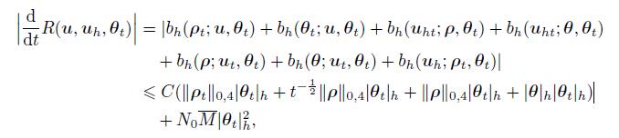 (66)
(66) and
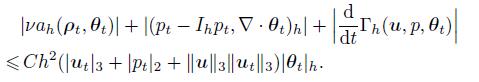 (67)
(67) Substituting (66) and (67) into (65) and combining with ν−1
 (68)
(68) Rearranging terms in (68) gives
 (69)
(69) Multiplying both sides of (69) by t and integrating it with respect to t,with the result (64),we have
 (70)
(70) Let σ(t) = max
 (71)
(71) which can derive the result (55) directly.
Taking vh = θt in (57),we have
 (72)
(72) Using Lemmas 1 and 5,we can obtain
 (73)
(73) Similar to (67),it holds
 (74)
(74) Substituting (73)-(74) into (72),we have
 (75)
(75) Multiplying both sides of (75) by t,integrating it with respect to t,and using (71),we have
 (76)
(76) Furthermore,we can derive
 (77)
(77) The desired result (56) follows from (77),and the proof is completed.
Theorem 2 Under the assumptions of Theorem 1,we have
 (78)
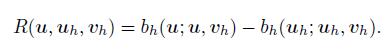
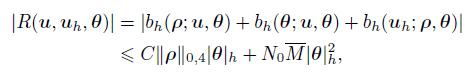
(78) Proof Subtracting (21) from (1),for all vh ∈ Vh,we obtain the error equation,i.e.,
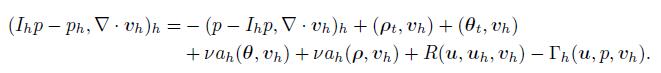 (79)
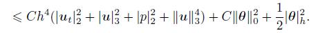
(79) By (24),(25) and Lemma 5,we have
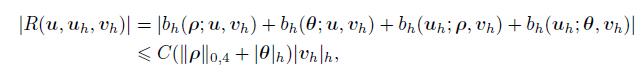 (80)
(80) and
 (81)
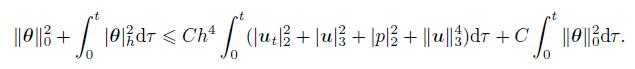
(81) Combining (79)-(81) and Theorem 1,we have
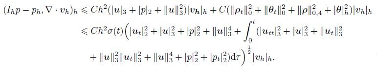 (82)
(82) Using the discrete inf-sup condition,we deduce

which implies the desired result. The proof is completed.
5 Superconvergent resultsNow,we start to introduce the post-processing operators (Π2h,I2h)[13] such that
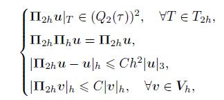 (83)
(83) 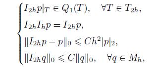 (84)
(84) where Q1(T) and Q2(T) are the spaces of the bilinear and quadratic functions on T ∈ T2h,respectively. We have the following superconvergent results.
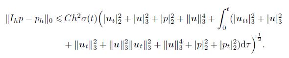
Theorem 3 Under the assumptions of Theorem 1,we have
 (85)
(85)  (86)
(86) Proof Noticing that
 (87)
(87) by (83) and interpolation error estimates,we have
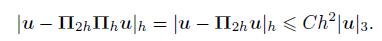 (88)
(88) Consequently,it follows from (83) and the result (56) of Theorem 1 that
 (89)
(89) which implies the result (85).
Similarly,we can derive the result (86). The proof is completed.
6 Numerical experimentIn this section,we present a numerical example to confirm our theoretical analysis.
To get enough accuracy,we use the linearly extrapolated Crank-Nicolson time-stepping scheme (see Ref. [26]) to perform the numerical experiment.
Consider the problem (1)−(4) on Ω = [0, 1]2,the exact solutions are

Now,we divide the domain into m × n uniform rectangles and obtain the errors of the velocity u and the pressure p in the broken H1-norm and the L2-norm at different time with m×n = 8×12,16 × 24,32 × 48,64 × 96,respectively.
The numerical results at different time and values of ν are listed in Tables 1−6. For convenience,we just plot the exact solutions u,p and the FEM solutions uh,ph at t = 1 with ν = 1 (see Figs. 2-4).


|
| Fig. 2 Diagrams of exact solutions u1 and u2 at t = 1 with ν = 1 |
|
|

|
| Fig. 3 Diagrams of FEM solutions uh1 and uh2 at t = 1 with ν = 1 |
|
|

|
| Fig. 4 Diagrams of exact solution p and FEM solution ph at t = 1 with ν = 1 |
|
|
It can be seen from Tables 1−6 that |u − uh|h and 


| [1] | Bernardi, C., & Raugel, G. A conforming finite element method for the time-dependent NavierStokes equations. SIAM Journal on Numerical Analysis, 22, 455-473 (1985) |
| [2] | He, Y. N. Optimal error estimate of the penalty finite element method for the time-dependent Navier-Stokes equations. Mathematics of Computation, 74, 1201-1216 (2005) |
| [3] | John, V., & Kaya, S. A finite element variational multiscale method for the Navier-Stokes equations. SIAM Journal on Scientific Computing, 26, 1485-1503 (2005) |
| [4] | Li, J., He, Y. N., & Chen, Z. X. A new stabilized finite element method for the transient Navier-Stokes equations. Computer Methods in Applied Mechanics and Engineering, 197, 22-35 (2007) |
| [5] | He, Y. N., & Sun, W. W. Stabilized finite element method based on the Crank-Nicolson extrapolation scheme for the time-dependent Navier-Stokes equations. Mathematics of Computation, 76, 115-136 (2007) |
| [6] | Shan, L., & Hou, Y. R. A fully discrete stabilized finite element method for the time-dependent Navier-Stokes equations. Applied Mathematics and Computation, 215, 85-99 (2009) |
| [7] | Chen, G., Feng, M. F., & He, Y. N. Finite difference streamline diffusion method using nonconforming space for incompressible time-dependent Navier-Stokes equations. Applied Mathematics and Mechanics (English Edition), 34, 1083-1096 (2013) |
| [8] | Crouzeix, M., & Raviart, P. A. Conforming and nonconforming finite element methods for solving the stationary Stokes equations I. Analyse Numérique, 7, 33-75 (1973) |
| [9] | Shi, D. Y., & Wang, H. M. The Crouzeix-Raviart type nonconforming finite element method for the nonstationary Navier-Stokes equations on anisotropic meshes. Acta Mathematicae Applicatae Sinica, 30, 145-156 (2014) |
| [10] | Ye, X. Superconvergence of nonconforming finite element method for the Stokes equations. Numerical Methods for Partial Differential Equations, 18, 143-154 (2002) |
| [11] | Shi, D. Y., & Pei, L. F. Superconvergence of nonconforming finite element penalty scheme for Stokes problem using L2 projection method. Applied Mathematics and Mechanics (English Edition), 34, 861-874 (2013) |
| [12] | Wang, X. S., & Ye, X. Superconvergence analysis for the Navier-Stokes equations. Applied Numerical Mathematics, 41, 515-527 (2002) |
| [13] | Liu, H. P., & Yan, N. N. Superconvergence analysis of the nonconforming quadrilateral linearconstant scheme for Stokes equations. Advances in Computational Mathematics, 29, 375-392 (2008) |
| [14] | Shi, D. Y., & Yu, Z. Y. Superclose and superconvergence analysis of a low order nonconforming mixed finite element method for stationary Stokes equations with damping (in Chinese). Acta Mathematica Scientia, 33 (2013) |
| [15] | Ciarlet, P. G. The Finite Element Method for Elliptic Problems, North-Holland, Amsterdam (1978) |
| [16] | Girault, V. and Raviart, P. A. Finite Element Method for Navier-Stokes Equations: Theory Algorithms, Springer-Verlag, Berlin/Heidelberg (1987) |
| [17] | Heywood, J. G., & Rannacher, R. Finite element approximation of the nonstationary NavierStokes problem I:regularity of solutions and second-order error estimates for spatial disretization. SIAM Journal on Numerical Analysis, 19, 275-311 (1982) |
| [18] | Rannacher, R., & Turek, S. Simple nonconforming quadrilateral Stokes element. Numerical Methods for Partial Differential Equations, 8, 97-111 (1992) |
| [19] | Ming, P. B. Nonconforming Element vs Locking Problem (in Chinese), Ph. D. dissertation, Chinese Academy of Sciences, Beijing (1999) |
| [20] | Xu, X. J. On the accuracy of nonconforming quadrilateral Q1 element approximation of NavierStokes problem. SIAM Journal on Numerical Analysis, 38, 17-39 (2000) |
| [21] | Hu, J., Man, H. Y., & Shi, Z. C. Constrained nonconforming rotated Q1 element for Stokes flow and planar elasticity (in Chinese). Mathematica Numerica Sinica, 27, 311-324 (2005) |
| [22] | Shi, D. Y., Ren, J. C., & Gong, W. A new nonconforming mixed finite element scheme for the stationary Navier-Stokes equations. Acta Mathematica Scientia, 31B, 367-382 (2011) |
| [23] | Shi, D. Y, & Ren, J. C Nonconforming mixed finite element approximation to the stationary Navier-Stokes equations on anisotropic meshes. Nonlinear Analysis:Theory. Methods and Applications, 71, 3842-3852 (2009) |
| [24] | Lu, X. L., & Lin, P. Error estimate of the P1 nonconforming finite element method for the penalized unsteady Navier-Stokes equations. Numerische Mathematik, 115, 261-287 (2010) |
| [25] | Wang, J. L., Si, Z. Y., & Sun, W. W. A new error analysis of characteristics-mixed FEMs for miscible displacement in porous media. SIAM Journal on Numerical Analysis, 52, 3000-3020 (2014) |
| [26] | Ingram, R. A new linearly extrapolated Crank-Nicolson time-stepping scheme for the NavierStokes equations. Mathematics of Computation, 82, 1953-1973 (2013) |