 2016, Vol. 37
Shanghai University
Article Information
- WU Jian, Q. RU C., ZHANG Liang, WAN Ling
- Geometrical shape of in-plane inclusion characterized by polynomial internal stress field under uniform eigenstrains
- Applied Mathematics and Mechanics (English Edition), 2016, 37(9): 1113-1130.
- http://dx.doi.org/10.1007/s10483-016-2130-6
Article History
- Received Feb. 17, 2016
- Revised May. 13, 2016


2. Department of Mechanical Engineering, University of Alberta, Alberta T6G 2G8, Canada;
3. State Key Laboratory of Structural Analysis for Industrial Equipment, Dalian University of Technology, Dalian 116024, China
The influence of the geometrical shape of an inclusion is studied on the internal stress field inside an inhomogeneous or homogenous inclusion in an infinite elastic plane under the uniform stress-free eigenstrains imposed within the inclusion. In spite of the extensive studies on this topic, especially for elliptical inclusions[1-12], little effort has been made to establish a general relation between the degree of the non-uniformity of the internal stress field and the geometrical shape of the inclusion. In particular, although it is well-known that ellipse is the only inclusion shape which achieves a uniform internal stress field under uniform eigenstrains[13], it seems unclear that what inclusion shapes will lead to a polynomial internal stress field given by a finite-degree polynomial of the spatial coordinates. Clearly, a polynomial internal stress field enjoys physical and mathematical simplicity compared with other more complicated non-uniform internal stress fields. Therefore, it is of great interest to identify the inclusion shapes which can achieve a polynomial internal stress field.
The present paper aims to determine the geometrical shape of an inclusion, whose internal stress field under uniform eigenstrains is polynomial. The problem is formulated in Section 2, and discussed in three different cases, i.e., an inhomogeneous inclusion with a different elastic modulus from the surrounding matrix, an inhomogeneous inclusion with the same shear modulus but a different Poisson's ratio from the surrounding matrix, and a homogeneous inclusion with the same elastic modulus as the surrounding matrix. The relation between the inclusion shape and the degree of the non-uniformity of the internal stress field is established. Several specific examples are given in Section 3, and the main conclusions are summarized in Section 4.
2 Inclusion shapes characterized by polynomial internal stress fieldConsider a linear elastic infinite plane with no remote loading at infinity, containing a subdomain of an unknown shape under the arbitrarily prescribed uniform stress-free eigenstrains $\left( \varepsilon _{xx}^{*}, \varepsilon _{yy}^{*}, \varepsilon _{xy}^{*} \right)$. The subdomain is occupied by an elastic inclusion, whose elastic modulus can be either identical to or different from that of the surrounding matrix. Our purpose is to determine the inclusion shape whose internal stress field caused by the prescribed uniform eigenstrains $\left( \varepsilon _{xx}^{*}, \varepsilon _{yy}^{*}, \varepsilon _{xy}^{*} \right)$ is given by the polynomial of the spatial coordinates $x$ and $y$ (see Fig. 1). Here, the inclusion is called the $l$th-order inclusion shape if its shape is defined by a polynomial mapping function of the degree $l$. In this paper, the trivial case of a circular inclusion is not considered, and $l$ is a positive integer. In Fig. 1, $S_2$ is the subdomain, within which the uniform stress-free eigenstrains $\left( \varepsilon _{xx}^{*}, \varepsilon _{yy}^{*}, \varepsilon _{xy}^{*} \right)$ are prescribed, $S_1$ is its supplement to the elastic plane, and $\Gamma$ is the interface between $S_1$ and $S_2$ which defines the inclusion shape. Throughout the present paper, the subscripts 1 and 2 denote the quantities in $S_1$ and $S_2$, respectively.

|
| Fig. 1 Inclusion of arbitrary shape in infinite plane |
|
|
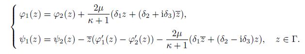
It is well-known[14] that the displacements and stresses in a linear elastic body can be given by two analytic functions $\varphi(z)$ and $\psi(z)$ and their conjugate functions with $z= x+ {\rm i}y$, i.e.,

where the superscript $'$ denotes derivatives, and $\mu$ is the elastic shear modulus. In the plane strain, $\kappa = 3-4\nu$, while in the plane stress, $\kappa= (3-\nu)/(1+\nu$), where $\nu$ is Poisson's ratio. The resultant force on the left-side of an arbitrary arc $PQ$ is[14]

Therefore, from the first equations in Eq.(1) and Eq.(2), the continuity conditions of the displacement and the traction along the interface between $S_1$ and $S_2$ and the zero-stress condition at infinity give

where

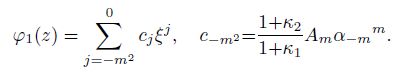
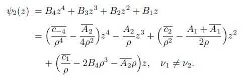
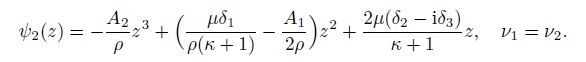
In the present paper, we will study what inclusion shapes can lead to an internal stress field given by a polynomial. It is seen from Eq.(1) that the internal stress field is given by the $n$th-degree polynomial if and only if the two potentials $\varphi_2(z$) and $\psi_2(z$) are polynomials of the degree not higher than ($n+1$), and at least one of the two potentials is a non-trivial ($n$+1)th-degree polynomial with a non-zero ($n$+1)th-degree coefficient. In particular, the two polynomials $\varphi_2(z$) and $\psi_2(z$) can have different degrees. Therefore, without loss of generality, inside the inclusion, we assume

where $m$ and $n$ are two finite non-negative integers, and

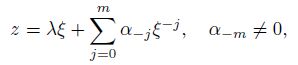
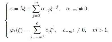
$A_0, \, A_1, \, \cdots, \, A_m$ and $B_0, \, B_1, \, \cdots, \, B_n$ are complex constants. To identify the inclusion shape giving the polynomial internal stress field given by Eq.(5) and determine the relation between the two polynomials in Eq.(5), we recall that the exterior of the unknown inclusion shape can be mapped onto the exterior of a unit circle by a conformal mapping[15]

where $\lambda$ is a real number, and $\alpha_0$, $\alpha_{-1}$, $\cdots$ are complex constants. $\alpha_0$ can determine the location of the inclusion, while the size of the inclusion can be decided by the amplitude of any one coefficient such as $\lambda$. Throughout the present paper, the trivial case of a circular inclusion is not considered, and then the lowest power of $\xi$ in Eq.(6) is strictly negative. For many practical problems, the mapping function (6) is often given or approximately given by a finite polynomial which only contains a finite number of terms. Therefore, the present study is restricted to the inclusion shape defined by the following polynomial mapping function:

where $l$ is a finite positive integer, and the associated inclusion shape here is called an $l$th-order inclusion shape. In particular, the polynomial mapping function (7) defines a one-to-one correspondence between the inclusion boundary in the $z$-plane and the unit circle in the $\xi$-plane. Here, the polynomial mapping (7) is analytical in the exterior of the unit circle including its boundary, and no singularity point of the mapping (7) can appear in the exterior of the unit circle or on its boundary. Once the unknown coefficients $\alpha_0$, $\alpha_{-1}$, $\alpha_{-2}, \;\cdots, \;\alpha_{-l}$ in Eq.(7) are determined so that the boundary conditions in Eq.(3) can be met with the polynomial complex potentials $\varphi_2(z$) and $\psi_2(z$) in Eq.(5), the shape of the inclusion can be determined.
For an inclusion undergoing the uniform eigenstrains ($\varepsilon_{xx}^*$, $\varepsilon_{yy}*$, and $\varepsilon_{xy}^*$), from the first and second equations in Eq.(3), on the boundary of the inclusion, we can express the complex potentials $\varphi_1(z$) and $\psi_1(z)$ in $S_1$ by the complex potentials $\varphi_2(z)$ and $\psi_2(z)$ in $S_2$, i.e.,

It is noticed that, in the exterior of the unit circle, when $z \to \infty$ and $\xi \to \infty$, from the third equation in Eq.(3), $\varphi_1(z)$ and $\psi_1(z)$ are analytic outside the unit circle and bounded at infinity in the $\xi$-plane. Therefore, $\varphi_1(z)$ and $\psi_1(z)$ can be given by the Laurent series as follows:

Similarly, $\varphi'_1(z)$ (the derivative of $\varphi_1(z)$ with respect to $z$) in the $\xi$-plane can be given by
 (10)
(10) where $h_j$ can be determined by
 (11)
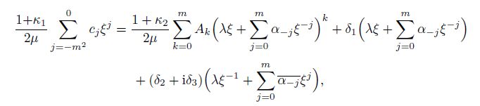
(11) In what follows, the inclusion shape which achieves the polynomial internal stress field (5) under the uniform eigenstrains $(\varepsilon _{xx}^{*}, \varepsilon _{yy}^{*}, \varepsilon _{xy}^{*})$ can be derived based on the two interface conditions in Eq.(8) for three different cases, depending on whether $\mu_1= \mu_2$ and $\nu_1 =\nu_2$. Actually, since the mapping (7) can be applied not only to the exterior of the unit circle but also to its boundary in the $\xi$-plane, we can apply the mapping (7) to the interface conditions in Eq.(8) with $\varphi_2$($z$) and $\psi_2$($z$) given by Eq.(5), and equate the coefficients of each power of $\xi$ on both sides of Eq.(8) along the boundary of the unit circle in the $\xi$-plane.
2.1 Inhomogeneous inclusion with ${ \mu}_{\bf 1}{\bf \ne} { \mu}_{\bf 2}$ and ${ \nu}_{\bf 1}{\bf \ne} { \nu}_{\bf 2}$Let us consider an inclusion with different elastic moduli $\mu$ and $\nu$, where $\mu_1 \ne \mu_2$, and $\nu_1 \ne \nu_2$. First, we consider the simple case when the internal stresses are constants, i.e., $n = 0$. Then,

in Eq.(5). Substituting Eqs.(5) and (9) into Eq.(8), viewing the highest power of $\xi$, we can get $l = 1$ and
 (13)
(13) which is the definition of an elliptical inclusion shape in the $z$-plane[5]. Moreover, it is well-known that an elliptical inhomogeneous inclusion under the uniform eigenstrains can give uniform internal stresses[16]. Therefore, the internal stresses of an inhomogeneous inclusion under uniform eigenstrains are all constants if and only if the inclusion shape is an ellipse.
Now, let us examine whether or not any higher $l$th-order non-elliptical inhomogeneous inclusion shapes (defined by a finite integer $l> 1$) exist, which can achieve a non-uniform polynomial internal stress field (max$(m, N) > 1$). Substituting Eqs.(5) and (7) into the first equation in Eq.(8) yields the following inclusion boundary:
 (14)
(14) where

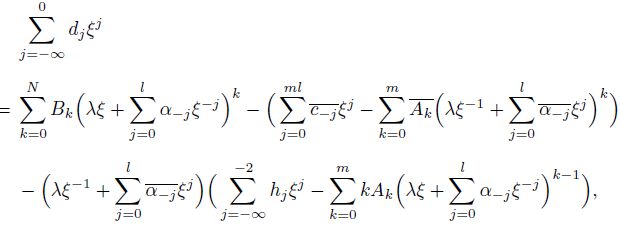
From Eq.(14), one can see that the highest orders of $\xi$ on the right-hand side are $m$, $ml-l+1$, $Nl$, $1$, and $l$ (or zero when $\delta_2+{\rm i}\delta_3 = 0$). To eliminate the highest power of $\xi$ on the right-hand side of Eq.(14), let

Then, one gets $N \leqslant1$, which gives a uniform stress field. Thus, for a non-uniform polynomial internal stress field, one needs $m > 1$. When $m > 1$ and $ l > 1$, one gets

Similarly, the lowest orders of $\xi$ on the right-hand side are $-ml$, $-(l+m-1)$, $-N$, $-l$, and $-1$ (or zero when $\delta_2+{\rm i}\delta_3 = 0$). Clearly, when $m > 1$ and $ l > 1$, one gets

Therefore, from Eq.(14), one gets

From the second equation in Eq.(8), one gets
 (15)
(15) where

From Eq.(15), one can see that the highest powers of $\xi$ on the right-hand side in every term are $N$, $ml$, $ml$, $l-2$, and $l+m-1$. Therefore, one gets $N = ml$ unless $c_{-ml} = A_m\alpha_{-l}^m$, by which the highest power $ml$ can be eliminated. From $ml-l+1 = Nl$ and $N = ml$, one gets $l = 1$, which is in contradiction with the previous condition $l > 1$. Therefore, the non-uniform polynomial stress field does not exist unless $c_{-ml} = A_m\alpha_{-l}^m$. When $c_{-ml} = A_m\alpha_{-l}^m$, from Eq.(14), one gets $\kappa_2\mu_1 = \kappa_1\mu_2$ and
 (16)
(16) Substituting Eq.(16) into the second equation of Eq.(8) yields

Since $\mu_1 > 0$, $\mu_2 > 0$, and $\kappa_1 > 0$, the coefficients of $\psi_2$ and $\overline z \varphi_2'$ in the above equation are nonzero. Viewing the highest power of $\xi$ in the above equation and noticing $A_m \ne 0$, $B_N \ne 0$, and $\alpha_{-l} \ne 0$, one gets $N = m+l-1$. From

one gets $l = 1$, which is in contradiction with the previous assumption $l > 1$. Therefore, it is concluded that the non-uniform polynomial internal stress field cannot be achieved by any non-elliptical inhomogeneous inclusion with the finite $l$th-order shape under the uniform stress-free eigenstrains with $\mu_1 \ne \mu_2$ and $\nu_1 \ne \nu_2$.
Therefore, for an inhomogeneous inclusion ($\mu_1 \ne \mu_2$, $\nu_1 \ne \nu_2$) defined by a polynomial mapping (7) which achieves a polynomial internal stress field under the uniform stress-free eigenstrains, the only possible inclusion shape is an ellipse, and the associated polynomial internal stress field is actually uniform. In what follows, however, it will be shown that the non-elliptical inclusion shapes defined by a polynomial mapping (7) can achieve a polynomial internal stress field if the inclusion has the same shear modulus as the matrix ($\mu_1 = \mu_2 = \mu$) no matter whether $\nu_1 = \nu_2$.
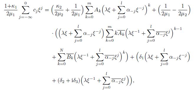
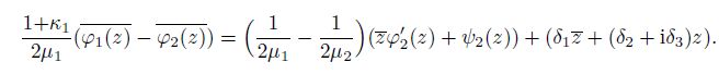
2.2 Inhomogeneous inclusion with ${ \mu}_{\bf 1}{\bf =} { \mu}_{\bf 2}$ and ${ \nu}_{\bf 1}{\bf \ne} { \nu}_{\bf 2}$The inhomogeneous inclusions which have the same shear moduli but different Poisson's ratios from the surrounding matrix have been studied in composite materials[17]. Let us now examine such inhomogeneous inclusions, where $\mu_1 = \mu_2$, and $\nu_1 \ne \nu_2$. Under the condition $\mu_1 = \mu_2 = \mu$, on the boundary of an inclusion, we can reduce Eq.(8) as follows:
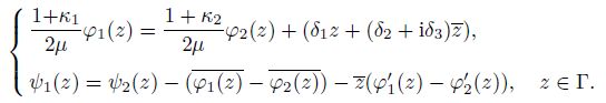 (17)
(17) Now, let us derive the inclusion shape in two respective cases, depending on whether $\delta_2+{\rm i}\delta_3 \ne 0$.
(i) Uniform eigenstrains with $\delta_2+{\rm i}\delta_3 \ne 0$
Substituting Eqs.(5), (7), and (12) into the first equation in Eq.(17), and viewing the highest and lowest powers of $\xi$ on both sides, since $A_m \ne 0$, one gets $l = m$. Thus,
 (18)
(18)  (19)
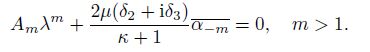
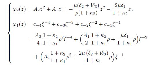
(19) First, we consider the case $m > 1$ in Eq.(5) for an inhomogeneous (non-elliptical) inclusion with $\mu_1 = \mu_2$ and $\nu_1 \ne \nu_2$. Substituting Eqs.(5), (9), (18), and (19) into Eq.(17), and equating the coefficients of the highest power of $\xi$ on both sides, since $A_m \ne 0$ and $B_n \ne 0$, one gets $N = (n+1) = m^2$. Then, we can conclude that the inclusion whose internal stress field given by the $n$th-degree polynomial $(n = m^2-1)$ has the $m$th-order inclusion shape. Furthermore, the coefficients $A_m$ and $B_N$ are not independent to confirm the existence of the non-zero solutions of $\lambda$ and $\alpha_{-m}$. It can be seen from Eqs.(5), (9), (17), (18), and (19) that, when $m>1$,
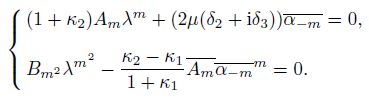 (20)
(20) Since $m > 0$, the first equation in Eq.(20) can be rewritten as the first equation in the following equation:
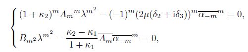 (21)
(21) where $m>1$. In Eq.(21), one gets two homogenous linear equations with two unknowns $(\lambda^m)^m$ and $\overline {\alpha_{-m}}^m$. Since both $\lambda$ and $\alpha_{-m}$ are non-zero, to have non-zero solutions, the determinant of the coefficient matrix of Eq.(21) must be zero, i.e.,
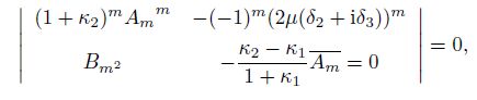 (22)
(22) where $m>1$. Therefore, one gets
 (23)
(23) Moreover, when $m > 1$, it can be proved that, if the inclusion has the $m$th-order shapes, the associated internal stress field can be given by the $n$th-degree polynomial with $n = m^2-1$. Actually, since both $\lambda$ and $\alpha_{-m}$ are non-zero, it is seen from Eq.(20) that $A_m \ne 0$ and $B_N \ne 0$, which is consistent with the basic assumption of Eq.(5). Then, from the third equation in Eq.(1), one can see that the degree of the polynomial internal stress field can be determined by $\psi_2'$ with

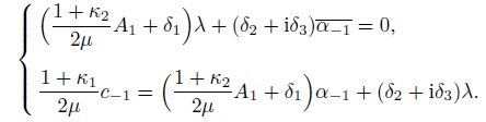
Next, we consider the case $m = 1$ in Eq.(5) for an inhomogeneous inclusion with $\mu_1 = \mu_2$ and $\nu_1 \ne \nu_2$. When $m = 1$, it follows from $l = m$ or the first equation in Eq.(17) that, the inclusion shape is an ellipse. From the second equation in Eq.(17), one gets that the internal stresses are constant, in agreement with the well-known conclusions in Ref.[16]. When $A_1 \ne 0$ and $B_1 \ne 0$, equating the coefficients of $\xi$ and $1/\xi$ on both sides of the first equation in Eq.(17), when $m=1$, one gets
 (24)
(24) Substituting the second equation in Eq.(24) and Eqs.(5), (9), and (19) into the second equation in Eq.(17) and equating the coefficients of $\xi$ on both sides, one gets
 (25)
(25) Viewing the first equations in Eqs.(24) and (25), to have non-zero $\lambda$ and $\alpha_{-1}$, one gets
 (26)
(26) Moreover, one needs to prove that the non-zero $\lambda$ and $\alpha_{-1}$ can give a non-zero uniform internal stress field. From the first equations in Eqs.(24) and (25), one gets $A_1 = B_1 = 0$ only if
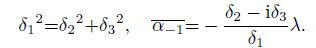 (27)
(27) Thus, in this case, the inclusion shape can be defined by
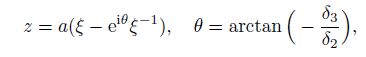 (28)
(28) where $a$ is a real number, and $\alpha_{0}$, measuring the axis movement, is ignored. Equation (28) maps a line segment (a crack) in the $z$-plane to a unit circle in the $\xi$-plane (see Fig. 2). Therefore, it is not considered as an inclusion shape, and not studied in the present paper.

|
| Fig. 2 Transformation from inclusion shapes to line segments |
|
|
At last, we consider the case $m = 0$ in Eq.(5). From the first equation in Eq.(17), it can be seen that the inclusion shape is an ellipse with

From the second equation in Eq.(17), it can be seen that

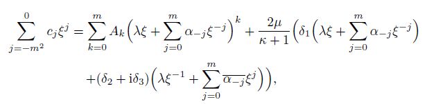
Therefore, it has been proved that, for an inhomogeneous inclusion with $\mu_1 = \mu_2 = \mu$ and $\nu_1 \ne \nu_2$ undergoing $\delta_2 + {\rm i}\delta_3 \ne 0$, the internal stress field is the polynomial of the degree $m^2-1$ if and only if the inclusion has an $m$th-order inclusion shape. Moreover, in this case, when $| { \xi } | = 1, $ the coefficients on the right-hand side of Eqs.(5), (7), and (9) satisfy
 (29)
(29) 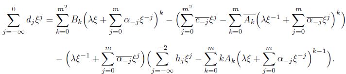 (30)
(30) Clearly, from Eqs.(29) and (30), it can be seen that, in the case that the power of $\xi$ is larger than zero, without considering the location of the inclusion and rigid-body displacement, there are $m(m+1)$ complex equations with $m(m+1)+1$ unknowns, i.e., $B_1$, $B_2$, $\cdots$, $B_{m^2}$, $\lambda$, and $\alpha_{-1}$, $\alpha_{-2}$, $\cdots$, $\alpha_{-m}$. In particular, it can be seen from the first equation in Eqs.(29) and (30) that one needs to know all coefficients of $\varphi_2$ to determine the normalized shape of the inclusion. In addition, if the amplitude $\lambda$ is given, one can have the exact inclusion shape. Therefore, once one chooses the value of $\lambda$, the shape of an inclusion can be identified from Eqs.(29) and (30). In particular, the coefficients $\alpha_{-1}$, $\alpha_{-2}$, $\cdots, $ $\alpha_{-m}$ can be determined by the first equation in Eqs.(29) and (30), and the coefficients $B_1$, $B_2$, $\cdots$, $B_{m^2}$ can be determined by the second equation in Eqs.(29) and (30).
In summary, for an inhomogeneous inclusion with

under the uniform eigenstrains with $\delta_2 + {\rm i}\delta_3 \ne 0$, we can obtain the internal stress field given by the polynomials of the degree $m^2-1$ if and only if the inclusion has an $m$th-order inclusion shape, and the coefficients of the highest power of two internal stress potentials $\varphi_2(z)$ and $\psi_2(z)$ must satisfy either Eq.(23) (when $m > 1$) or Eq.(26) (when $m = 1$) to ensure the existence of a non-zero solution.
(ii) Uniform eigenstrains with $\delta_2+{\rm i}\delta_3 = 0$
The thermal effect is a common cause of mismatch between the inclusion and the matrix. It can lead to a subdomain undergoing the expansion with $\delta_2+{\rm i}\delta_3 = 0$. When $\delta_2+{\rm i}\delta_3 = 0$, from the first equation in Eq.(17), and viewing Eqs.(7) and (9), one gets Eq.(5), where $m = 1$, and
 (31)
(31) Substituting Eq.(31) into the second equation in Eq.(17), since $B_N \ne 0$, one gets

and
 (32)
(32)  (33)
(33) From Eq.(33), one can see that the inclusion shape only depends on the elastic modulus of the inclusion $\kappa_2$. In addition, in Eq.(32), if $\alpha_{-n-1} \ne 0$, one gets $B_{n+1} \ne 0$.
Therefore, for an inhomogeneous thermal inclusion with

under the thermal eigenstrains with $\delta_2+{\rm i}\delta_3 = 0$, the internal stress field is a polynomial of the degree $n$ if and only if the inclusion has an $(n+1)$th-order inclusion shape, and the internal stress potentials $\varphi_2(z)$ and $\psi_2(z)$ are a linear function given by Eq.(31) and an $(n+1)$th-order polynomial, respectively. From Eq.(33), it is seen that the relation between the inclusion shape and the internal stress field is independent of Poisson's ratio of the surrounding matrix.
2.3 Homogeneous inclusion with ${ \mu}_{\bf 1}{\bf = }{ \mu}_{\bf 2}$ and ${ \nu}_{\bf 1}{\bf =} { \nu}_{\bf 2}$When the inclusion has the same elastic modulus as the surrounding matrix, Eq.(8) can be further simplified as follows:
 (34)
(34) In the cases of either the thermal inclusions ($\delta_2+{\rm i}\delta_3 = 0$) or the elliptical inclusions ($m = 1$ or $m = 0$), it can be readily verified that the solution can be directly obtained by letting $\kappa_1 = \kappa_2 = \kappa$ in Eqs.(24)--(26) and (31)--(33) from the previous results.
Therefore, let us only consider the case when

which cannot be obtained directly by letting $\kappa_1 = \kappa_2 = \kappa$ from the previous results in Subsection 2.2 since the highest powers of $\xi$ are different. Viewing Eqs.(5), (7), and (10), and equating the coefficients of the highest power of $\xi$ on both sides in Eq.(34), since $A_m \ne 0$, one gets $l = m$, and
 (35)
(35)  (36)
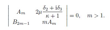
(36) From the second equation in Eq.(34), viewing Eqs.(10), (11), and (34), and equating the coefficients of the highest power of $\xi$ on both sides, since

one gets

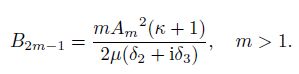
and
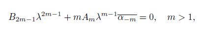 (37)
(37) where $B_{2m-1} \ne 0$. The coefficients $A_m$ and $B_{2m-1}$ are not independent to confirm the existence of the non-zero solutions of $\lambda$ and $\alpha_{-m}$. Viewing Eqs.(36) and (37), one gets two homogenous linear equations with two unknowns $\lambda^{2m-1}$ and $\lambda^{m-1}\overline{\alpha_{-m}}$. Since both $\lambda$ and $\alpha_{-m}$ are non-zero, to have non-zero solutions, the determinant of the coefficient matrix must be zero, i.e.,
 (38)
(38) Therefore, one gets
 (39)
(39) Moreover, one needs to ensure that the $m$th-order inclusion shape can lead to the internal stress field given by the $n$th-order polynomial ($n = 2m-2$). When $m > 1$, because both $\lambda$ and $\alpha_{-m}$ are non-zero in Eq.(35), from Eqs.(36) and (37), one gets

Then, from the third equation in Eq.(1), one can see that the degree of the internal stress field can be determined by $\psi_2'$ when $N = n+1 > m$. Since $B_N \ne 0$, the internal stress field is given by the $n$th-order polynomial of the spatial coordinates. In this case, the coefficients of the right-hand side of Eqs.(5), (7), and (9) can be determined by
 (40)
(40) 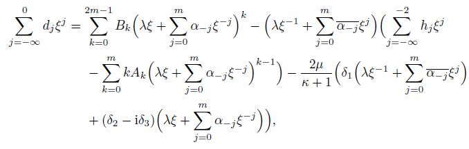 (41)
(41) where $| \xi | = 1.$
Clearly, from Eqs.(40) and (41), it can be seen that in the case that the power of $\xi$ is larger than zero, without considering the location of the inclusion and rigid-body displacement, there are $3m-1$ complex equations with $3m$ unknowns, i.e., $B_1\, B_2, \, \cdots, \, B_{2m-1}$, $\lambda$, and $\alpha_{-1}, \, \alpha_{-2}, \, \cdots, \alpha_{-m}$. In particular, it can be seen that, from Eq.(40), one needs to know all coefficients of $\varphi_2$, to determine the normalized shape of the inclusion. In addition, if the amplitude $\lambda$ is given, one can have the exact inclusion shape. Therefore, once one chooses the value of $\lambda$, the shape of an inclusion can be identified from Eq.(40). In particular, the coefficients $\alpha_{-1}, \, \alpha_{-2}, \, \cdots, \alpha_{-m}$ can be determined by Eq.(40), and the coefficients $B_1\, B_2, \, \cdots, \, B_{2m-1}$ can be determined by Eq.(41).
In summary, when $\delta_2+{\rm i}\delta_3 \ne 0$, the internal stress field of a homogenous inclusion is given by the polynomial of the degree $2(m-1)$ if and only if the inclusion has an $m$th-order inclusion shape, and the coefficients of the highest power of two internal stress potentials $\varphi_2(z)$ and $\psi_2(z)$ must satisfy Eq.(39) (when $m > 1$) or Eq.(26) (when $m = 1$) to ensure the existence of the non-zero solutions. Therefore, compared with an inhomogeneous inclusion whose internal stresses are given by the polynomial of the same degree, a homogenous inclusion is of a higher-order shape. In other words, with the same order of inclusion shapes, an inhomogeneous inclusion has a higher-degree polynomial internal stress field.
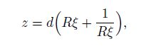
3 Examples and discussion 3.1 Homogenous inclusion of uniform internal stresses (${ n}{\bf = 0}$)First, let us consider a homogenous inclusion of uniform internal stresses as a verification example. As we have discussed above, in this case, the inclusion shape is elliptical, and $m \leqslant1$ in Eq.(5). Furthermore, assume that

where $R$ is a real constant, and $R > 1$. Let $\kappa_1 = \kappa_2 = \kappa$ in Eq.(26). Then, one gets

which agrees with that in Ref.[7]. Thus, in the next, we can verify our results in comparison with the results in Ref.[7]. From the first equation in Eq.(24) in the present paper, one gets

If we select $\lambda = dR$, where $d$ is the half distance between two foci, ignoring the axis movements in the $\xi$-plane, one gets[7]

From the second equation in Eq.(24), one gets
 (42)
(42) Noticing
 (43)
(43) from the second equation in Eq.(29), one gets in Eq.(9)
 (44)
(44) which agrees with the Laurent series in Ref.[7].
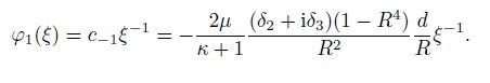
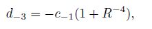
3.2 Thermal rectangular inclusion of rounded cornersIn practical applications, an important geometrical shape of thermal inclusions is rectangle[2]. From Ref.[7], the exterior of an approximate rectangle of the rounded corners can be mapped onto the exterior of a unit circle by the following mapping function with $l = 3$ (see Fig. 3):
 (45)
(45)

|
| Fig. 3 Approximate rectangles with rounded corners |
|
|
where $k$ and $c$ are real constants. Thus, for an inhomogeneous inclusion with the same shear modulus but a different Poisson's ratio from the sounding matrix, from Eqs.(31)--(33), equating the coefficients of powers higher than 0, one gets
 (46)
(46) Let $\kappa_2 = \kappa$. Then, Eq.(46) is the same as that in Ref.[7]. From Eq.(46), one can see that the internal stress field of a thermal inhomogeneous rectangular inclusion of rounded corners, which has the same shear modulus but a different Poisson's ratio from the sounding matrix, is independent of Poisson's ratio of the surrounding matrix.
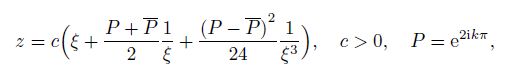
3.3 Inhomogeneous or homogenous inclusion of internal stresses given by eighth-degree polynomial $({ n}{\bf = 8})$From the results in Section 2, it can be seen that, even though the degree of the polynomial of the internal stress field is the same as that of a homogeneous inclusion, the order of the shape of an inhomogeneous inclusion with $\mu_1 = \mu_2 = \mu$ and $\nu_1 \ne \nu_2$ is different from that of a homogenous inclusion. In addition, these two types of inclusions can only give the internal stresses given by the polynomials of certain degrees. Actually, except constants, the eighth-degree polynomial is of the lowest degree which can define the internal stress field for both inhomogeneous and homogenous inclusions. Therefore, in this section, we identify the inclusion shape which gives the internal stress field defined by the eighth-order polynomial, i.e.,

From the previous discussion in Section 2, one knows that, for an inclusion whose internal stresses are given by the eighth-degree polynomial, an inhomogeneous inclusion with $\mu_1 = \mu_2 = \mu$ and $\nu_1 \ne \nu_2$ has a third-order inclusion shape, and a homogeneous inclusion has a fifth-order inclusion shape. Two typical inclusion shapes are hypotrochoids with cusps (see Fig. 4), i.e.,
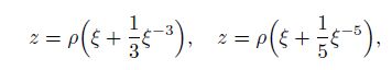 (47)
(47)

|
| Fig. 4 Shapes of inclusions with internal stresses given by eighth-degree polynomials: left, shape of inhomogeneous inclusion with $\mu_1 = \mu_2 = \mu$ and $\nu_1 \ne \nu_2$; right, shape of homogeneous inclusion |
|
|
where $\rho$ is a real constant.
3.4 Effect of different Poisson's ratios (${ \mu}_{\bf 1}{\bf =}{ \mu}_{\bf 2}{\bf =} { \mu}$ and ${ \nu}_{\bf 1}{\bf \ne } { \nu}_{ \bf 2})$In this section, we discuss the errors caused by a simplified homogenous model, which ignores the difference in Poisson's ratios of the inclusion and the matrix by setting $\nu = \nu_2$. All results shown below are under the plane strain conditions.
(i) Elliptical inclusions
First, let us consider an elliptical inclusion (first-order inclusion shape) as follows:
 (48)
(48) where $R$ is a real constant, $R > 1$, $d$ is the half distance between two foci. In this case, the internal stress field of an inclusion is constant for both the inhomogeneous model with $\mu_1 = \mu_2 = \mu$ and $\nu_1 \ne \nu_2$ and the simplified homogenous model with $\nu = \nu_2$. From Eq.(25), we have the inhomogeneous model expressed by
 (49)
(49) From Eq.(1), the internal stress field can be determined by the derivatives of the potentials $\varphi_2$ and $\psi_2$. From Eq.(49), it can be seen that the stress potential $\varphi_2$ is independent of Poisson's ratio of the surrounding matrix, which indicates that the summation of $\sigma_{xx}$ and $\sigma_{yy}$ in the inclusion is independent of Poisson's ratio of the surrounding matrix. Thus, we only consider the effect of different Poisson's ratios on $\psi_2'$. For simplicity, let us consider the uniform eigen-strain $\varepsilon_{xx}^* \ne 0$ with $\varepsilon_{yy}^* = \varepsilon_{xy}^* = 0$. In this case, $\delta_1 = \delta_2 \ne 0$, $\delta_3 = 0$, and $\psi_2'$ is a real constant. When $R = 2$ and $ \nu_2 = 0.35$, comparing the homogeneous model ($\nu = \nu_2$) with the inhomogeneous model ($\mu_1 = \mu_2 = \mu$, $\nu_1 \ne \nu_2)$), from Eq.(49), we have that the relative error of $\psi_2'$ is $12.7\%$ when $\nu_1 = 0.2$ and 15.3% when $\nu_1 = 0.5$. The parameter $R$ measures the shape of the ellipse (see the left figure of Fig. 5), and the effect of $R$ is shown in the right figure of Fig. 5. From Fig. 5, it can be seen that the relative error of $\psi_2'$ increases monotonously with the increase in $R$ and tends to a constant when $R$ is very large. Therefore, the relative error of $\psi_2'$ increases with the increase in the relative length of the minor axis of an ellipse, and reaches the maximum when an ellipse tends to a circle. Moreover, the relative error of $\psi_2'$ is of the same order of the magnitude as the relative error of Poisson's ratio $(|\nu_2-\nu_1|/|\nu_1|)$.

|
| Fig. 5 Dependence of relative error of homogenous model on elliptical shape parameter $R$ |
|
|
(ii) Hypotrochoidal inclusions
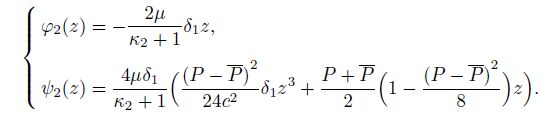
Now, let us consider the Hypotrochoid of the second-order inclusion shape
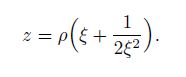 (50)
(50) In this case, the stress distribution is different between the inhomogeneous model with $\mu_1 = \mu_2 = \mu$ and $\nu_1 \ne \nu_2)$ and the homogeneous model with $\nu = \nu_2$. For the inhomogeneous model with $\mu_1 = \mu_2 = \mu$ and $\nu_1 \ne \nu_2$, from Eq.(29), one gets
 (51)
(51) Since
 (52)
(52) from Eq.(30), one gets
 (53)
(53) Moreover, for the homogeneous model with $\nu = \nu_2$, the stress potential $\varphi_2$ is the same as that in Eq.(51). Therefore, the summation of $\sigma_{xx}$ and $\sigma_{yy}$ in the inclusion is independent of Poisson's ratio of the surrounding matrix. From Eq.(41), for the homogenous model, one gets
 (54)
(54) From Eq.(51), it can be seen that the stress potential $\varphi_2$ is independent of Poisson's ratio of the surrounding matrix, which indicates that the summation of $\sigma_{xx}$ and $\sigma_{yy}$ in the inclusion is independent of Poisson's ratio of the surrounding matrix. Actually, from Eqs.(8) and (17), it can be seen that the coefficients in $\varphi_2$ are independent of $\kappa_1$. Thus, for an inclusion whose internal stresses are defined by a polynomial, the summation of $\sigma_{xx}$ and $\sigma_{yy}$ within the inclusion is independent of Poisson's ratio of the surrounding matrix.
For simplicity, let us consider the uniform eigen-strain $\varepsilon_{xx}^* \ne 0$ with $\varepsilon_{yy}^* = \varepsilon_{xy}^* = 0$. In this case, $\delta_1 = \delta_2 \ne 0$, and $\delta_3 = 0$. Compared with the inhomogeneous model with $\mu_1 = \mu_2 = \mu$ and $\nu_1 \ne \nu_2$, the relative error of $\psi_2'$ obtained by the homogeneous model ($\nu = \nu_2$) is shown in Figs. 6 and 7. In all the calculations, we set $\nu_2 = 0.35$. First, let Poisson's ratio $\nu_1$ be $0.350\, 1$ and the maximum relative error inside an inclusion obtained by the homogeneous model be $7\%$, which are caused by the relative error of Re$(\psi_2')$. The maximum relative error of Re$(\psi_2')$ is two orders of magnitude higher than the relative error of Poisson's ratio ($(|\nu_2-\nu_1|/|\nu_1|)$), since at some points Re$(\psi_2')$ obtained by the inhomogeneous model closes to zero. Therefore, we consider the error of the mean value of Re$(\psi_2')$ in the entire inclusion. The relative error of the mean value of Re$(\psi_2')$ is $0.03\%$, which is of the same order of magnitude as the relative error of Poisson's ratio. Thus, the inhomogeneous model reduces to the homogeneous model, which verifies our results. In Figs. 6 and7, we let $\nu_1 = 0.2$ in Fig. 6 and $\nu_1 = 0.5$ in Fig. 7. From Figs. 6 and 7, it can be seen that the relative error can be very large at some points in the inclusion. However, we can calculate the relative error of the mean value of $\psi_2'$. The results show that the relative error of the mean value of Re$(\psi_2')$ is $4.6\%$ and the relative error of the mean value of Im$(\psi_2')$ is $3.7\%$ when $\nu_1 = 0.2$, while the relative error of the mean value of Re$(\psi_2')$ is $6.5\%$ and the relative error of the mean value of Im$(\psi_2')$ is $5.2\%$ when $\nu_1 = 0.5$. Therefore, in this case, the relative error of the mean value of $\psi_2'$ is one order of magnitude lower than the relative error of Poisson's ratio.

|
| Fig. 6 Relative error of Re$(\psi_2')$ in inclusion when $\nu_1 = 0.2$, and $\nu_2 = 0.35$ |
|
|

|
| Fig. 7 Relative error of Im$(\psi_2')$ in inclusion when $\nu_1 = 0.5$, and $\nu_2 = 0.35$ |
|
|
Although the polynomial internal stress field enjoys physical and mathematical simplicity, it has attracted little attention in the study of Eshelby's problem of an inclusion under uniform eigenstrains. For an inhomogeneous or homogenous inclusion under the uniform stress-free eigenstrains in an infinite elastic plane, the present work studies what inclusion shapes will lead to a polynomial internal stress field. Here, we confine ourselves to the inclusion shapes defined by the polynomial mapping functions which map the exterior of the inclusion onto the exterior of a unit circle. Several examples are presented to illustrate the methods and results, and the effects of different Poisson's ratios between the inclusion and the surrounding matrix are discussed in detail. The specific conclusions achieved in the present work are as follows:
(i) For an inhomogeneous inclusion with a different shear modulus and a different Poisson's ratio from the surrounding matrix, the only possible finite-order inclusion shape, which achieves a polynomial internal stress filed, is an ellipse, and the associated internal stress field is uniform.
(ii) For an inhomogeneous inclusion with the same shear modulus but a different Poisson's ratio from the surrounding matrix, under the uniform arbitrary eigenstrains with $\delta_2+{\rm i}\delta_3 \ne 0$, the internal stresses are given by the polynomial of the degree $(m^2-1)$ if and only if the inclusion shape is defined by an $m$th-degree polynomial mapping function.
(iii) For a homogeneous inclusion under the uniform arbitrary eigenstrains with $\delta_2+{\rm i}\delta_3 \ne 0$, the internal stresses are given by the polynomial of the degree $2(m-1)$ if and only if the inclusion shape is defined by an $m$th-degree polynomial mapping function.
(iv) For an inclusion having the same shear modulus as the surrounding matrix, under the uniform thermal eigenstrain with $\delta_2+{\rm i}\delta_3 = 0$, the internal stresses are given by the polynomial of the degree $n$ if and only if the inclusion shape is defined by an $(n+1)$th-degree polynomial mapping function, and the relation between the inclusion shape and the internal stress field is independent of Poisson's ratio of the surrounding matrix.
| [1] | Sendeckyj, & G., P Elastic inclusion problems in plane elastostatics. International Journal of Solids and Structures, 6, 1535-1543 doi:10.1016/0020-7683(70)90062-4 (1970) |
| [2] | H, u, & S., M Stress from a parallelepipedic thermal inclusion in a semispace. Journal of Applied Physics, 66, 2741-2743 doi:10.1063/1.344194 (1989) |
| [3] | Ni, wa, H, ., Ya, gi, H, ., Tsuchikawa, H, ., and, Kato, & M Stress distribution in an aluminum interconnect of very large scale integration. Journal of Applied Physics, 68, 328-333 doi:10.1063/1.347137 (1990) |
| [4] | Fa, ux, D., A., Downes, J., R., and, Oreilly, & E., P A simple method for calculating strain distributions in quantum-wire structures. Journal of Applied Physics, 80, 2515-2517 doi:10.1063/1.363034 (1996) |
| [5] | R, u, C., Q. and Schiavone, & P On the elliptic inclusion in anti-plane shear. Mathematics and Mechanics of Solids, 1, 327-333 doi:10.1177/108128659600100304 (1996) |
| [6] | Rodin, & G., J Eshelby's inclusion problem for polygons and polyhedral. Journal of the Mechanics and Physics of Solids, 44, 1977-1995 doi:10.1016/S0022-5096(96)00066-X (1996) |
| [7] | R, u, & C., Q Analytic solution for Eshelby's problem of an inclusion of arbitrary shape in a plane or half-plane. ASME Journal of Applied Mechanics, 66, 315-322 doi:10.1115/1.2791051 (1999) |
| [8] | L, i, S, ., Sauer, R, ., and, Wang, & G., A circular inclusion in a finite domain I the Dirichlet-Eshelby problem. Acta Mechanica, 179, 67-90 (2004) |
| [9] | L, iu, & Y., W. and Fang Q. H Plane elastic problem on the rigid lines along a circular inclusion. Applied Mathematics and Mechanics (English Edition), 26(12), 1585-1594 (2005) |
| [10] | J, in, X., Q., Ke, er, L., M., and, Wang, & Q New Green's function for stress field and a note of its application in quantum-wire structures. International Journal of Solids and Structures, 40, 3788-3798 (2009) |
| [11] | Z, ou, W, ., H, e, Q, ., Huang, M, ., and, Zheng, & Q Eshelby's problem of non-elliptical inclusions. Journal of the Mechanics and Physics of Solids, 58, 346-372 doi:10.1016/j.jmps.2009.11.008 (2010) |
| [12] | Ch, en, & Y., Z Closed form solution and numerical analysis for Eshelby's elliptic inclusion in plane elasticity. Applied Mathematics and Mechanics (English Edition), 35(7), 863-874 (2014) |
| [13] | Horgan, & C., O Anti-plane shear deformation in linear and nonlinear solid mechanics. SIAM Review, 37, 53-81 doi:10.1137/1037003 (1995) |
| [14] | England, A. H. Complex Variable Methods in Elasticity, Wiley InterScience, London (1971) |
| [15] | Kantorovich, L. V. and Krylov, V. I. Approximate Methods of Higher Analysis, Wiley InterScience, London (1958) |
| [16] | Eshelby, & J., D The determination of the elastic field of an ellipsoidal inclusion and related problems. Proceedings of the Royal Society A:Mathematical, Physical and Engineering Science, 241, 376-396 doi:10.1098/rspa.1957.0133 (1957) |
| [17] | Rooney, F., and Ferrari, & M On the St. Venant problem for inhomogeneous circular bars. SME Journal of Applied Mechanics, 66, 32-40 doi:10.1115/1.2789165 (1999) |