 2016, Vol. 37
Shanghai University
Article Information
- XIE Dan, JIAN Kailin, WEN Weibin
- Global interpolating meshless shape function based on generalized moving least-square for structural dynamic analysis
- Applied Mathematics and Mechanics (English Edition), 2016, 37(9): 1153-1176.
- http://dx.doi.org/10.1007/s10483-016-2126-6
Article History
- Received Dec. 19, 2015
- Revised Apr. 7, 2016


2. State Key Laboratory of Coal Mine Disaster Dynamics and Control, Chongqing University, Chongqing 400044, China;
3. College of Engineering, Peking University, Beijing 100871, China
The analysis of structural dynamics is an essential and arduous task during the period of product design. Many practical engineering problems are always abstracted as a set of partial differential equations associated with the boundary and initial conditions. Due to the difficulty to obtain the analytical solutions, many effective numerical methods have been developed to satisfy the requirements of the engineering applications. However, most of the presented methods are limited to meshes, e.g., the finite element method (FEM) and the boundary element method (BEM).
In recent decades, meshless or meshfree methods[1-2] have become attractive alternatives in computational mechanics, where the approximate solutions are obtained based on a set of scattered nodes in the whole domain, instead of meshes or elements. Therefore, there is no need for mesh generation and mesh refinement in actual engineering problems. Several meshless methods have been successfully formulated and applied for various static and dynamic problems[3-10], such as the elementfree Galerkin (EFG) method, the reproducing kernel particle method (RKPM), the meshless local Petrov-Galerkin (MLPG) method, and the radial point interpolation method (RPIM).
The EFG method is one of the most popular meshless methods due to its high accuracy and simple implementation. Belytschko et al.[3] proposed the EFG method firstly by combining the Galerkin weak form of partial differential equations (PDEs) and the moving least-square (MLS) approximation[11-12] for elasticity problems. The superiority of the EFG method has been confirmed in a series of problems[12-25]. However, the EFG method based on the MLS always presents low accuracy for complex essential boundary conditions. Atluri et al.[26] proposed the generalized MLS (GMLS) to formulate the shape functions on the basis of the MLPG method, where the derivatives of the displacements were treated as independent variables and introduced into the interpolating scheme. The results show that the GMLS approximation presents higher accuracy than the MLS. For the structures whose derivative variables can be imposed at the same point like displacements, the approximations of the GMLS are more preferable. Mirzaei and Schaback[27] used the GMLS approximations to the direct meshless local Petrov-Galerkin (DMLPG) method to overcome the shortages within the MLPG based on the MLS. Valencia et al.[28] adopted the GMLS in the EFG method to analyze the influence of the selectable parameters by a one-dimensional (1D) beam in bending problems
However, the GMLS approximation is the non-interpolating algorithm just as the MLS. Its shape functions do not satisfy the Kronecker delta property. Besides, with the more complex expressions compared with the MLS, the imposition of the boundary conditions of the EFG method based on the GMLS becomes more difficult. As the best knowledge of the authors, a little amount of work on the EFG method with the GMLS approximation has been reported, particularly for two-dimensional (2D) dynamic problems. Some special approaches have been introduced to solve the problems of the boundary conditions, such as the penalty method[19-21] and the Lagrange multiplier method[4, 12]. However, the selection of the penalty factor for the penalty method mainly depends on numerical experiments and researcher's experience. Sometimes, the inappropriate selection of the penalty factor may make the system ill-conditioned[21]. The Lagrange multiplier method always introduces additional unknowns, which are not directly related to the solutions in the analysis. Zhang et al.[21], Ren and Cheng[29], Cheng et al.[30], Zhang et al.[31], and Sun et al.[32] formulated the interpolating element-free Galerkin (IEFG) method based on the MLS interpolates, where singular weight functions or orthogonal basis functions were used. The aforementioned methods may be feasible for the EFG method based on the MLS, while for the GMLS, they are difficult to be used.
Instead of dealing with modified weight or basis functions, Chen et al.[33-34] proposed the transformation technique in early time, and successfully extended the studies to nonlinear problems by use of the RKPM. Recently, Garijo et al.[35] adopted the later transformation in the EFG method based on the MLS. The results showed that it was very easy to impose the boundary conditions. However, the interpolating MLS shape function is limited to certain types of boundary conditions due to its low computational accuracy. Meanwhile, the interpolating nature of this method will lose its meaning when the derivative variables are included in the boundary conditions.
Given the high accuracy of the GMLS approximation and the convenience of the transformation method in the imposition of boundary conditions, a global interpolating GMLS (IGMLS) shape function is obtained by combining the transformation technique and the GMLS approximation. In this paper, an improved EFG method based on the global IGMLS is proposed. With a simple matrix transformation, the dynamic discretized equations of the proposed method is directly derived. For the proposed method, the shape functions possess a global interpolating property. Both the displacements and the derivative boundaries are imposed easily. Meanwhile, the actual values of the nodal variables rather than the nodal parameters are obtained directly from the discretized equations. Thus, the proposed method can avoid all computational loops for actual nodal variables in the conventional EFG method, and is easily compatible with other numerical algorithms. This is helpful in improving the computational efficiency of the structural dynamic analysis.
The beam and plate with the boundary conditions which are simplified from the practical engineering structures such as bridges and solar panels have been adopted for the numerical researches in different meshless methods[12, 36-47]. In this paper, the dynamic analyses of Euler beams and Kirchhoff plates with different boundary conditions and dynamic loads are conducted to validate the feasibility and effectiveness of the improved method.
The paper is organized as follows. In the next section, the formulation of the global IGMLS shape function is described in detail, and its interpolating property is analyzed theoretically. Based on the IGMLS, the dynamic discretized equations with the EFG method are formulated in Section 3. In Section 4, the numerical results of the Euler beams and the Kirchhoff plates for the modal and forced vibration analyses are given to validate the effectiveness of the proposed method. Lastly, some conclusions of this study are given in Section 5.
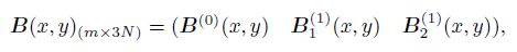
2 Shape functions of EFG method 2.1 Standard GMLS shape functionsConsider the 2D problem occupying a domain ${\Omega }$ with a set of scattered points ${ x}_{k} (x_{k}, \, y_{k} )$ $({ k=1, 2}, \cdots, {N})$, where ${N}$ is the number of the nodes in the support domain. The approximation of the field variable $w^h(x, y)$ can be expressed in terms of a polynomial basis ${ p}(x, y)$ and the vector of unknown parameters $ a$ as follows:


where $m$ is the number of the terms of the monomials in ${ p}(x, y)$.
The unknown $ a$ at any given point can be determined by minimizing the errors between the local approximations ($w^h(x_{k} , y_{k} )$ and its derivatives $\theta _x ^h(x_{k} , y_{k} )$ and $\theta _y ^h(x_{k} , y_{k} ))$ and the nodal parameters ($w_{k}, \; \theta _{xk}, $ and $\theta _{yk})$ at this point, i.e.,

where $\omega _{k} (x, y)$ is the local supported weight function expressed by

Take the following cubic spline weight function for example:

where

in which $d_{m{k}x} $ and $d_{m{k}y} $ are the sizes of the affected domain of the ${k}$th node in the $x$-direction and the $y$-direction, respectively. For 1D case, $d_{{ mk}} =N_{\rm S}\times c_{k} $, where $N_{\rm S}$ is the scale factor, and $c_{k} $ is the distance among the nodes in regular distribution.
The stationary of the function of the weighted residual $J$ with $ a$ is

Substituting Eq.(4) into Eq.(6) yields

Then, Eq.(7) can be rewritten in the matrix form as follows:

where

 (10)
(10)  (11)
(11) and

Substituting Eq.(8) into Eq.(1) yields the variable approximates by the GMLS as follows:
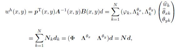 (12)
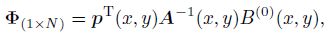
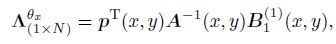
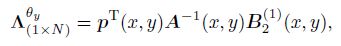
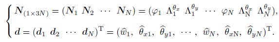
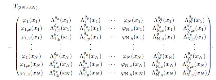
(12) where ${ \Phi} $ is the shape function matrix corresponding to the field variable, $\Lambda ^{\theta _x }$ and $\Lambda ^{\theta _y }$ are the shape function matrices corresponding to the first derivatives of the field variable, and $N$ is the matrix of the standard GMLS shape function for the 2D problem, i.e.,
 (13)
(13)  (14)
(14)  (15)
(15)  (16)
(16) Modify Eq.(10). Then, the order of the elements within Eq.(16) can be adjusted as follows:
 (17)
(17) The first and second derivatives of the standard GMLS shape function can be obtained by
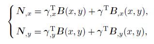 (18a)
(18a) 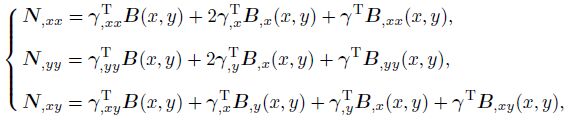 (18b)
(18b) where
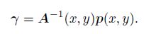 (19)
(19) According to the GMLS shape functions, the field variable and its derivatives at any point can be expressed by
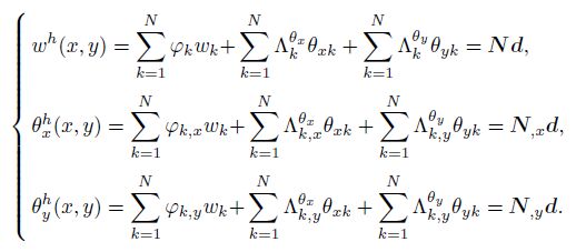 (20)
(20) Define $ U$ as the values of the actual nodal variables, i.e.,
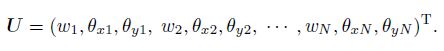 (21)
(21) Then, the relationship between the actual nodal variables and the nodal parameters (see Eq.(17)) can be written as follows:
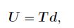 (22)
(22) where $T$ is the transformation matrix expressed by
 (23)
(23) Equation (20) can be expressed by the actual nodal variables as follows:
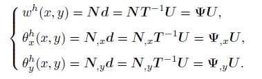 (24)
(24) Thus, the global IGMLS shape function $ \Psi $ and its derivatives ${ \Psi} _{, x} $ and ${ \Psi} _{, y} $ can be expressed by the GMLS shape functions as follows:
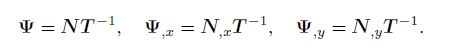 (25)
(25) The delta property is the notable feature of the IGMLS shape functions, which cannot be found in standard GMLS approximations. With Eqs (21)--(23), we can express the transformation matrix as follows:
 (26)
(26) According to Eqs.(25)--(26), we can rewrite the global IGMLS shape function $ \Psi $ as follows:
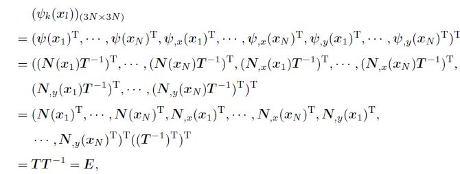 (27)
(27) where $ E$ is the unit matrix.
Consequently, Eq.(27) shows the Kronecker delta property of both the IGMLS shape functions and their derivatives. This is in agreement with the IGMLS approximation, where both the displacements and the derivatives are included in the interpolation.
The GMLS and IGML shape functions of the 1D problem with 11 nodes are shown in Fig. 1(a) and Fig. 1(b), respectively. The quartic spline weight function and the polynomial basis functions $(m=3.0)$ are used in this case.

|
| Fig. 1 Shape functions of 1D problem, where wave peaks correspond $N_i$ ($i=1, \, 2, \, \cdots, \, 11)$ from left to right |
|
|
For clarity, the shape functions at a single node are given in Fig. 2. GMLS-1 and IGMLS-1 are the denote shape functions of the field variable. GMLS-2 and IGMLS-2 denote the shape functions of the first derivative of this field variable. In Fig. 2, it can be noted that the GMLS shape functions and their derivatives have local supported features, while the IGMLS shape functions and the derivatives show the interpolating property in the whole domain.

|
| Fig. 2 Shape functions of signal node |
|
|
The shape functions of GMLS-1 and IGMLS-1 at the middle node with different scale factors are shown in Fig. 3. Figure 3(a) plots the shape functions with regular distributions, and Fig. 3(b) shows the shape functions the irregular distributions. We can see that the scale factor defines the size of the support domain in the GMLS, while indicates oscillations in the IGMLS.

|
| Fig. 3 Shape functions of field variable at middle node with different scale factors |
|
|
Figure 4 plots the GMLS and IGML shape functions at the middle node of the 2D structure with regular ${11}\times {11}$ scattered nodes. The quartic spline weight function and polynomial basis function with $m=6$ are used here. Similarly, the GMLS-1 and IGMLS-1 denote the shape functions of the field variable. The GMLS-21 and IGMLS-21 denote the shape functions of the first derivative of this field variable in the $x$-direction. GMLS-22 and IGMLS-22 denote the shape functions of the first derivative in the $y$-direction. Figure 4 shows that the shape functions of the 2D case have the same property as the 1D case.

|
| Fig. 4 Shape functions at middle node of 2D problem |
|
|
Consider a homogeneous and isotropic Kirchhoff plate defined in the domain $Z=\Omega \times(-h/2, h /2), \Omega \in {\mathbb{R}}^2$. Under the Cartesian coordinate system, the displacements of the plate in the $x$-, $y$-, and $z$-directions are denoted, respectively, as $u$, $v$, and $w$. $w$ is also the deflection of the plate in the domain $\Omega $. In the classical Kirchhoff's plate theory, the deflections of $w(x, y)$ can be independent variables, and the displacement fields of the plate are given by
 (28)
(28) The dynamic equilibrium equation of the plate expressed in a strong form is
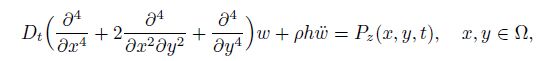 (29)
(29) where $\rho $ is the mass density, $h$ is the thickness of the plate, $P_z (x, y, t)$ is the lateral dynamic load, $t$ indicates the time, and $D_t$ is the flexural rigidity expressed by
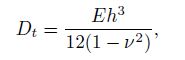 (30)
(30) in which $E$ and $\nu $ are Young's modulus and Poisson's ratio, respectively.
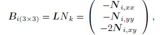
The geometric equation is
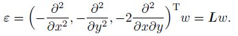 (31)
(31) The constitutive equation describes the relationship between the stresses and the strains in terms of the generalized Hooke's law, i.e.,
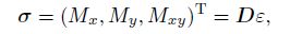 (32)
(32) where ${ \varepsilon}$ is the curvature or generalized strain vector, $ \sigma $ is the generalized stress vector including three components, i.e., the bending moments $M_x$ and $M_y$ and the twisting moment $M_{xy} $, and
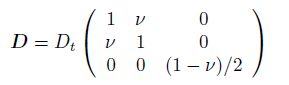 (33)
(33) is the constant matrix of the material property.
The natural and essential boundary conditions of the plate with four simply-supported edges are
 (34)
(34)  (35)
(35) where ${\Gamma}_u $ and ${\Gamma}_t$ denote the displacement boundary and the load boundary, respectively.
The initial conditions are
 (36)
(36) where both $\theta _x =\frac{\partial w}{\partial y}$ and $\theta _y =-\frac{\partial w} {\partial x}$ are the rotation angles.
3.2 Discretized equations based on GMLSThe Galerkin weak form of Eq.(29) can be written as follows:
 (37)
(37) where ${ P}=({P_x }\;\, {P_y }\;\, {P_z })^{\rm T}$ is the external load in the space. The penalty method is used for the imposition of the boundary conditions, and $\alpha $ is the penalty factor.
According to Eqs.(28) and (32), the weak form of Eq.(37) can be written further as follows:
 (38)
(38) Consider that the plate is scattered by a set of nodes in the space $\Omega $. Substituting Eq.(12) and Eq.(17) into Eq.(38), we can obtain the dynamic discretized equations of the Kirchhoff plate. For the forced vibration analysis, there is
 (39)
(39) where
 (40)
(40) The mass matrix, the node stiffness matrix, the node force vector, the penalty stiffness matrix, and the penalty force vector, respectively, are
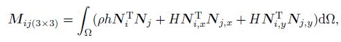 (41)
(41) 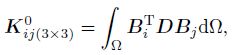 (42)
(42)  (43)
(43) 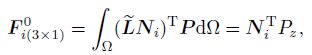 (44)
(44)  (45)
(45)  (46)
(46) where ${H}=\int_{\rm Z} {\rho z^2{\rm d}{\rm Z}=} \rho \int_{-h/2}^{h/2} {z^2{\rm d}{\rm Z}=} {\rho h^3} /{12}$ is the inertial mass moment for the homogeneous plate.
For the free vibration analysis, we have
 (47)
(47) where ${ d}(x, y, t)$ can be written as follows:
 (48)
(48) Substituting Eq.(48) into Eq.(47) yields the eigenvalue equations as follows:
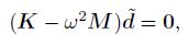 (49)
(49) where $\omega $ is the natural circular frequency, $\theta $ is the phase angle, and $\tilde { d}$ is the mode vector.
3.3 Discretized equations based on global IGMLSBased on the relationship of the shape functions between the GMLS and the IGMLS as Eq.(27), we have the modified stiffness matrix as follows:
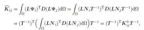 (50)
(50) the modified mass matrix as follows:
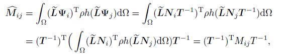 (51)
(51) and the modified force vector as follows:
 (52)
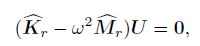
(52) Consequently, we have the modified eigenvalue equations
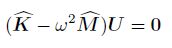 (53)
(53) and the modified forced vibration equations
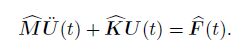 (54)
(54) Obviously, from the transformation matrix (see Eq.(25)), we can see that the solutions of the modified dynamic equations (see Eq.(53) and Eq.(54)) can be attributed to solve the matrices described in Eq.(41), Eq.(42), and Eq.(44). In this paper, the classic Gaussian quadrature with the background cells is adopted to conduct the integration. The specific integration expressions of matrices are
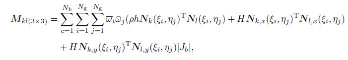 (55)
(55) 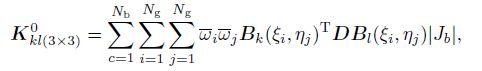 (56)
(56) 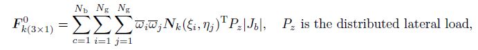 (57)
(57)  (58)
(58) where $N_{\rm b}$ is the number of the background cells, $\xi _i$ and $ \eta _j $ are the coordinates of the Gauss point in the $x$-direction and the $y$-direction, respectively, $N_{\rm g}$ is the Gauss point, $| { J_b }|$ is the Jacobi coefficient of the computational points, $\bar {\omega }_i \overline{\omega}_j $ is the weight coefficient for the 2D case, and ${ x}_{Qi} $ is the coordinate of the point where the external load is acted.
Based on the feature of the GMLS and the Kronecker delta property of the global IGMLS, both the deflections and rotation angles on the boundary conditions can be imposed directly by the straightforward imposition method as in the FEM. For the 1D problem, the essential boundary is a single point. For the 2D problem, the boundary is degraded into a set of points. The eigenvalue equations and forced vibration equations after imposition of the boundary conditions are
 (59)
(59) 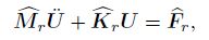 (60)
(60) where $\widehat { M}_r$, $ \widehat { K}_r $, and $\widehat { F}_r $ are the final modified mass matrix, the stiffness matrix, and the force vector, respectively, and the dimension of these matrices can be reduced due to the straightforward method.
4 Numerical resultsTo validate the feasibility of the proposed method for the dynamic analysis, in this paper, free and forced vibration analyses of the Euler beams and the Kirchhoff plates are conducted.
In Fig. 5(a), the simply-supported Euler beam is illustrated. The structure size is $L=10$ m and $b\times h=0.5\, {\rm m}\times 0.5\, {\rm m}$. The material properties are $E=2.0\times 10^{7}$~N$\cdot$m$^{-2}$ and $\rho $=10$^{3}$ kg$\cdot$m$^{-3}$.

|
| Fig. 5 Simply-supported Euler beam subjected to lateral concentrated load |
|
|
In Fig. 6, a square plate with four simply-supported edges is provided. The structure size and the material properties are $a\times b=10\, {\rm m}\times 10\, {\rm m}$, $h=0.05\, {\rm m}$, $E=2.0\times 10^{11}\, {\rm N}\cdot{\rm m}^{-2}$, $\upsilon =0.3$, and $\rho=8\times 10^{3}\, {\rm kg}\cdot{\rm m}^{-3}$.

|
| Fig. 6 Simply-supported Kirchhoff plate subjected to lateral concentrated load |
|
|
Both the standard GMLS and the global IGMLS are incorporated into the EFG method by the equidistantly distributed nodes. For the 1D case, four Gauss quadrature points are used in each cell, while 4$\times $4 Gauss points are used in each cell for the 2D case. The Penalty method is used in the GMLS, and the straightforward imposition method is used in the IGMLS. All cases are coded in the computer with Pentium(R) Dual-Core CPU E5300@2.60 GHz.
4.1 Modal analysisIn this section, the Euler beams and Kirchhoff plates are adopted to study the characteristics of the proposed method for the modal analysis. These characteristics include the condition numbers of the final modified matrices, the computational accuracy, the convergence rate, and the computational cost. Meanwhile, to investigate the advantage of the proposed method in the imposing essential boundary conditions, some cases are provided, i.e., the Euler beam simply-supported at both ends (Beam-SS), the beam with one end clamped and the other free (Beam-CF), the beam with one end clamped and the other simply-supported (Beam-CS), the beam clamped at both ends (Beam-CC), the Kirchhoff plate with four simply-supported edges (Plate-SSSS), and the plate with one edge clamped and others free (Plate-CFFF)
4.1.1 Modal analysis of Euler beamFirstly, the condition numbers of the stiffness and mass matrices in the dynamic discretized equations of both the GMLS method and the IGMLS method are calculated by the $L^{2}$ norm. For the GMLS method, 10$^{7}$ is adopted as the penalty factor. The number of the nodes (or degree-of-freedom (DOF)) of 21, 51, 101, and 201 and the scale factors of 2, 3, and 4 are discussed. For simplicity, only the results of Beam-SS and Beam-CC are plotted in Fig. 7.

|
| Fig. 7 Condition numbers of matrices in dynamic discretized equations of beam with IGMLS and GMLS methods |
|
|
From Fig. 7(a) and Fig. 7(b), we can see that the condition numbers of the stiffness matrix of Beam-SS are from 6 to 10 and the condition numbers of the mass matrix of Beam-SS are from 4 to 6. In Fig. 7(c) and Fig. 7(d), it is clear that the condition numbers of the stiffness matrix of Beam-CC are almost confined from 5 to 10, and the condition numbers of the mass matrix of Beam-CC are from 3 to 5. The matrix's condition number of the IGMLS method remains far below the GMLS for all node densities and scale factors. In addition, the influence of the scale factors on matrix's condition number of the IGMLS is much significant than the GMLS.
From the above results, we can obtain that the transformation technology greatly improve the ill-conditioned problem existing in the GMLS method and make the numerical calculation more stable.
Then, modal analyses of the Euler beam with four kinds of boundary conditions are conducted, where the beam is discretized by 51 regular nodes, and the scale factor is 2.0. Compared with the analytical solutions, the results of the first ten natural circular frequencies presented in Table 1 show the high accuracy of the proposed method, even for high-order frequencies.

|
Further, define $h$ as the average distance of the discretized nodes. Then, the computational accuracy can be evaluated by the relative error as follows:
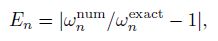 (61)
(61) where $\omega _n^{\rm num} $ and $\omega _n^{\rm exact}$ are the numerical and exact values of the $n$th circular frequency, respectively.
The convergence rates of both the IGMLS and GMLS methods are studied by the first two natural frequencies of Beam-SS. The curves in Fig. 8 show that the IGMLS and GMLS methods have almost the same high accuracy and the same convergence rate, except for some points with bigger errors due to the mismatching of the numbers of the nodes and the scale factors in the numerical calculation. In addition, the cases of Beam-CF, Beam-CS, and Beam-CC are also researched by authors. All results verify the high accuracy of the IGMLS method, and show that the transformation technology used in the IGMLS method has little influence on the computational accuracy of the modal analysis. Therefore, the proposed method can keep the high accuracy of the GMLS approximation well.

|
| Fig. 8 Comparisons of convergence rates of IGMLS and GMLS methods for Beam-SS |
|
|
The computational cost of the GMLS method and the IGMLS method can be evaluated by $R_{\rm CPU}=T_{\rm CPU{\_}IGMLS}/T_{\rm CPU{\_}GMLS}$, where $T_{\rm CPU{\_}IGMLS}$ and $T_{\rm CPU{\_}GMLS}$ are the calculated CPU time for the IGMLS method and the GMLS method, respectively. Four kinds of boundary conditions and two scale factors of 2.0 and 3.0 are considered (see Fig. 9). It can be noticed that the values of the ratio are mainly concentrated in [1.1, 1.4]. It can be seen that the CPU time of the IGMLS method is slightly higher than the GMLS method. However, the relation curves of the computational accuracy and the cost of these two methods plotted in Fig. 10 show that the computational cost of the IGMLS is lower than the GMLS method under the same computational accuracy.

|
| Fig. 9 Ratio of computational cost with different essential boundary conditions |
|
|

|
| Fig. 10 Computational accuracy versus CPU time with different essential boundary conditions |
|
|
The influence of the transformation matrix on the condition numbers of the final modified matrices are also studied by the cases of Plate-SSSS and Plate-CFFF. For the GMLS method, 10$^{12}$ is adopted as the penalty factor. The DOFs of the plate with $121({11}\times {11})$, $169 ({13}\times {13})$, $225 ({15}\times {15})$, and $289 ({17}\times {17})$ and the scale factors of 1.5, 2.0, and 2.5 are discussed.
Figures 11(b) and 11(d) show that the condition numbers of the mass matrices for both Plate-SSSS and Plate-CFFF are concentrated in [3.5, 4.5]. From Fig. 11(a) and Fig. 11(c), we can see that the condition numbers of the stiffness matrices are in [3.5, 4.5] for Plate-SSSS and [5, 6] for Plate-CFFF. Thus, the conclusions from the plate case for the condition number analyses are in agreement with the results from the beam.

|
| Fig. 11 Condition numbers of matrices in dynamic discretized equations of plate with IGMLS and GMLS methods |
|
|
In the modal analyses of Plate-CFFF and Plate-CFFF, the structure is discretized by 11$\times $11 regular nodes, and the scale factor is 2.0. The first ten natural circular frequencies calculated by the IGMLS method are presented in Table 2. Here, the values computed by the FEM with 100$\times $100 elements are considered as the ``analytical'' solutions. The results of the GMLS and MLS methods with the same number of nodes as the IGMLS method are also shown for the comparison.

|
Obviously, the data in Table 2 indicate that both the IGMLS method and the GMLS method have far higher accuracy than the standard MLS method. They can keep the high accuracy even for high order frequencies of the plate, which is the same as in the beam case. In addition, the modal analysis results are shown visually by the first eight mode shapes of Plate-CFFF, which are plotted in Fig. 12. Both bending vibration and torsional vibration can be seen clearly in these mode shapes. The first-, third-, and seventh-order mode shapes present the transverse bending vibration, and other mode shapes show varying degrees of torsional deformation.

|
| Fig. 12 First eighth order mode shapes of Plate-CFFF |
|
|
The computational accuracy of the IGMLS method for the plate is studied in the same way as the beam, where the square plate is discretized by the regular nodes of $121 ({11}\times {11})$, $169 ({13}\times {13})$, $225 ({15}\times {15})$, $289 ({17}\times {17})$, $361 ({19}\times {19})$, and $441 ({21}\times {21})$. Here, the low-order case (the first-order frequency) and the high-order case (the tenth-order frequency) are discussed in Fig. 13. Some results of the relative error are listed in Table 3.

|
| Fig. 13 Convergence rates of IGMLS and GMLS methods for plates |
|
|

|
The high accuracy of low- and high-order frequencies for both the IGMLS method and the GMLS method is shown clearly in Fig. 13. However, it seems that the convergence rates cannot be presented obviously by these curves. The main reason is the occurrence of some points with big errors due to the mismatching of the number of the nodes and the scale factors in the IGMLS or GMLS method. In fact, the same case occurs in the examples of the beams. However, the problem is more evident for the plate. Even though, the very similar tendency of the curves in Fig. 13 between the IGMLS method and the GMLS method can still be shown if these special points are not in consideration. Thus, the numerical results of plates validate again that, in the modal analysis, the proposed method can keep high accuracy and a similar rate of convergence as the GMLS method.
The CPU time is calculated in the same way as the beams. More data about the ratio of the CPU time for both the LGMLS and the GMLS methods are plotted in Fig. 14. The figure shows that the values of the ratio of Plate-SSSS and Plate-CFFF are mainly located in [1.0, 1.1] (see Fig. 14(a)) and in [1.0, 1.2] (see Fig. 14(b)), respectively. It indicates that both the methods have almost equivalent computational cost. In addition, it can be seen from Table 3 that the little change of the scale factors can lead to a big difference in the computational costs. Thus, a little scale factor is favorable for the improvement of the computational efficiency.

|
| Fig. 14 Ratio of computational cost with different scale factors |
|
|
The nodal variables in Eq.(60) are a function of both space and time. Based on the GMLS approximation and the IGMLS approximation, the equations discretized in space are obtained. In the time domain, assume that the time is scatted by the time step $\Delta {t}$, and the dynamic equations at the time ${t+}\Delta {t}$ is
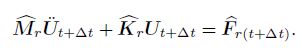 (62)
(62) At present, many kinds of methods, such as the Newmark scheme, the Houbolt scheme, the Wilson, and the central difference time integration, can be used to solve Eq.(62). The Newmark scheme, i.e.,
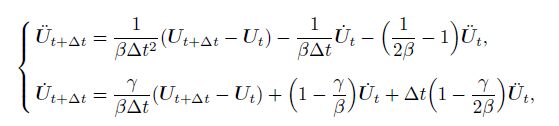 (63)
(63) is used in this paper. In the following numerical examples, $\beta ={3}/{4}$, and $\gamma ={1} /{2}$.
From Eq.(62), we can see that the notable advantage of the IGMLS method is that actual nodal variables can be obtained directly in every time loop. Thus, the proposed method can be easily compatible with the subprograms of the standard Newmark scheme, which is helpful for the computational efficiency.
The analytical solutions of the dynamic responses can be obtained easily. In this section, Beam-SS and Plate-SSSS (see Figs. 5 and 6) with the concentrated harmonic and constant loads (see Fig. 15) exerted at the midpoint are adopted for the forced vibration analysis.

|
| Fig. 15 Dynamic loads exerted at midpoint of beams or plates |
|
|
Consider Beam-SS discretized by 51 regular nodes. The harmonic load acted on the beam can be expressed as 1~000$\times f_{1}(t)$ with the forced frequency $w=5$~rad$\cdot$s$^{-1}$, and the constant load is 1~000$\times f_{2}(t)$.
Firstly, the influences of the time step and scale factors on the dynamic responses are investigated under the harmonic load. The results of the displacement responses at the midpoint with different time steps are plotted in Fig. 16. It can be seen that the time step of 0.01 s is proper for this case. Then, the value of 0.01 s is adopted as the time step for the further study of the scale factors. From Fig. 17, we can find that the scale factor has little influence on the displacement responses and the values from 2.0 to 4.0 are feasible.

|
| Fig. 16 Effects of time step on displacement response |
|
|

|
| Fig. 17 Effects of scale factor on displacement response |
|
|
Then, the time step of 0.01 s and the scale factor of 2.0 are adopted in the harmonic case. The results of both the IGMLS method and the GMLS method are given in Fig. 18. In the same way, the displacement responses of the constant load with the time step of 0.05 s and the scale factor of 2.0 are shown in Fig. 19. From Figs. 18 and 19, we can easily find that the displacement responses of the IGMLS method are highly consistent with the analytical solutions.

|
| Fig. 18 Displacement responses at midpoint of beam under harmonic load |
|
|

|
| Fig. 19 Displacement responses at midpoint of beam under constant load |
|
|
In the plate cases, the forced frequency of the harmonic load is 10$\, {\rm rad}\cdot{\rm s}^{-1}$, and the constant load is the same as the beam. The plate is discretized by regular 13$\times $13 nodes.
After similar numerical researches of the step time and scale factor as in the beam cases, the scale factor of 1.5 and the time step of 0.01 s are adopted for both kinds of dynamic loads. The responses of deflection at the point $(a/3, \, b/3)$ are analyzed. Figures 20 and Figures 21 provide the results of the harmonic load and the constant load, respectively.

|
| Fig. 20 Deflection responses of plate under harmonic load |
|
|
Figures 2-21 show that the IGMLS and GMLS methods compare favorably with the analytical solutions in the forced vibration analyses. The results confirm again the high accuracy property of the proposed method for the forced vibration analyses.

|
| Fig. 21 Deflection responses of plate under harmonic load |
|
|
Besides, the computational cost of the two methods (see Table 4) is calculated. Compared with the results of the modal analysis, we find that the computational efficiency of the IGMLS method is higher than that of the GMLS method in the forced vibration analyses.

In this study, an improved EFG method based on the global IGMLS is proposed for the structural dynamic analysis, where the IGMLS shape function is formulated by employing the transformation technology in standard GMLS approximations. The theoretical analyses verify the Kronecker delta property of the IGMLS shape function and its derivatives in the whole domain. The dynamic discretized equations of the proposed method are derived by the simple matrix transformation. The numerical simulations of the Euler beams and Kirchhoff plates with different boundary conditions and dynamic loads are performed to validate the proposed method. The main conclusions of this study are drawn as follows:
(i) For the proposed method, essential boundary conditions including both displacements and derivatives can be imposed by the straightforward method as in the FEM. The improved method is efficient in dealing with the boundary conditions which are confirmed by the dynamic analyses of the Euler beams and Kirchhoff plates with different boundaries.
(ii) Compared with the conventional EFG method, actual nodal variables can be obtained directly from the dynamic discretized equations. The proposed method can avoid cumbersome computational loops for every node, and is easily compatible with other numerical algorithms, by which the computational efficiency can be improved.
(iii) The introduction of the transformation matrix greatly improves the ill-conditioned feature of the standard GMLS method with a penalty factor, which ensures the better stability of the proposed method.
(iv) The transformation technology used in the IGMLS method has little influence on the computational accuracy and convergence rate compared with the GMLS. The numerical simulations show that the proposed method can provide very accurate natural frequencies even for the high-order and the high accuracy of the dynamic responses. The advantage in the computational accuracy is prominent when it is compared with some commonly used schemes, such as the conventional FEM and the EFG method based on the MLS method.
(v) The IGMLS and GMLS methods have almost the same computational cost for the modal analysis. While for forced vibration analyses, the computational efficiency of the IGMLS method is obviously higher than that of the GMLS method.
In summary, the proposed method based on the global IGMLS is convenient and stable to implement the comparison with the conventional EFG method. With the high accuracy and more acceptable time cost, the proposed method is more desirable for structural dynamic problems. In addition, not limited to the Euler beams and Kirchhoff plates mentioned in this paper, the proposed method can be applied to structures with any complicated shape and other high-order continuous problems, especially when the solution accuracy is the main objective.
| [1] | Fries, T. P. and Matthies, H. G. Classification and Overview of Meshfree Methods, Technical University Braunschweig, Brunswick, Germany (2004) |
| [2] | Belytschko, T, Kronganz, Y, Organ, D, Fleming, M, & Krysl, P Meshless methods:an overview and recent developments. Computer Methods in Applied Mechanics and Engineering, 139, 3-47 doi:10.1016/S0045-7825(96)01078-X (1996) |
| [3] | Belytschko, T, ., L, u, Y., Y., and, Gu, & L Element-free Galerkin methods. International Journal for Numerical Methods in Engineering, 37, 229-256 doi:10.1002/(ISSN)1097-0207 (1994) |
| [4] | Dolbow, J., and Belytschko, & T An introduction to programming the meshless element free Galerkin method. Archives of Computational Methods in Engineering, 5, 207-241 doi:10.1007/BF02897874 (1998) |
| [5] | L, iu, W., K., J, un, S, ., Zhang, Y., F., Ad, ee, J, ., and, Belytschko, & T Reproducing kernel particle methods for structural dynamics. International Journal for Numerical Methods in Engineering, 38, 1655-1679 doi:10.1002/(ISSN)1097-0207 (1995) |
| [6] | Atluri, S., N. and Zhu, & T A newmeshless local Petrov-Galerkin (MLPG) approach in computational mechanics. Computational Mechanics, 22, 117-127 doi:10.1007/s004660050346 (1998) |
| [7] | G, u, Y., T. and Liu, & G., R A local point interpolation method for static and dynamic analysis of thin beams. Computer Methods in Applied Mechanics and Engineering, 190, 5515-5528 doi:10.1016/S0045-7825(01)00180-3 (2001) |
| [8] | L, iu, G., L. and Li, & X., W Mesh free method based on local cartesian frame. Applied Mathematics and Mechanics (English Edition), 27(1), 1-6 (2006) |
| [9] | Zhang, Z., Q., Zh, ou, J., X., Wa, ng, X., M., Zhang, Y., F., and, Zhang, & L h-adaptivity analysis based on multiple scale reproducing kernel particle method. Applied Mathematics and Mechanics (English Edition), 26(8), 1064-1071 (2005) |
| [10] | Ze, ng, Q., H. and Lu, & D., T Galerkin meshless methods based on partition of unity quadrature. Applied Mathematics and Mechanics (English Edition), 26(7), 893-899 (2005) |
| [11] | Lancaster, P., and Salkauskas, & K Surfaces generated by moving least squares methods. Mathematics of Computation, 37, 141-158 doi:10.1090/S0025-5718-1981-0616367-1 (1981) |
| [12] | Noguchi, H, ., Kawashima, T, ., and, Miyamura, & T Element free analyses of shell and spatial structures. International Journal for Numerical Methods in Engineering, 47, 1215-1240 doi:10.1002/(ISSN)1097-0207 (2000) |
| [13] | Krysl, P., and Belytschko, & T Analysis of thin plates by the element-free Galerkin method. Computational Mechanics, 17, 26-35 doi:10.1007/BF00356476 (1995) |
| [14] | Ouatouati, A., E. and Johnson, & D., A A new approach for numerical modal analysis using the element-free method. International Journal for Numerical Methods in Engineering, 46, 1-27 doi:10.1002/(ISSN)1097-0207 (1999) |
| [15] | L, i, G., and Belytschko, & T Element-free Galerkin method for contact problems in metal forming analysis. Engineering Computations, 18, 62-78 doi:10.1108/02644400110365806 (2001) |
| [16] | Ventura, G, ., X, u, J., X., & and, Belytschko T. A vector level set method and new discontinuity approximation for crack growth by EFG. International Journal for Numerical Methods in Engineering, 54, 923-944 doi:10.1002/(ISSN)1097-0207 (2002) |
| [17] | Bobaru, S., and Mukherjee, & S Meshless approach to shape optimization of linear thermoelastic solids. International Journal for Numerical Methods in Engineering, 53, 765-796 doi:10.1002/(ISSN)1097-0207 (2002) |
| [18] | Singh, & I., V Meshless EFG method in three-dimensional heat transfer problems:a numerical comparison, cost and error analysis. Numerical Heat Transfer Applications, 45, 199-220 (2004) |
| [19] | Singh, & I., V Parallel implementation of the EFG method for heat transfer and fluid flow problems. Computational Mechanics, 34, 453-463 doi:10.1007/s00466-004-0590-0 (2004) |
| [20] | L, iu, L, ., Ch, ua, L., P., and, Ghista, & D., N Element-free Galerkin method for static and dynamic analysis of spatial shell structures. Journal of Sound Vibration, 295, 388-406 doi:10.1016/j.jsv.2006.01.015 (2006) |
| [21] | Zhang, Z, ., H, ao, S., Y., Li, ew, K., M., and, Cheng, & Y., M The improved element-free Galerkin method for two-dimensional elastodynamics problems. Engineering Analysis with Boundary Elements, 37, 1576-1584 doi:10.1016/j.enganabound.2013.08.017 (2013) |
| [22] | Singh, I., V., Tanaka, M, ., and, Endo, & M Thermal analysis of CNT-based nano-composites by element free Galerkin method. Computational Mechanics, 39, 719-728 doi:10.1007/s00466-006-0061-x (2007) |
| [23] | Am, ir, K., and Mohammad, & R., H A new method for meshless integration in 2D and 3D Galerkin meshfree methods. Engineering Analysis with Boundary Elements, 34, 30-40 doi:10.1016/j.enganabound.2009.07.008 (2010) |
| [24] | B, ui, T., Q., Nguyen, M., N., and, Zhang, & C., Z A moving Kriging interpolation-based element-free Galerkin method for structural dynamic analysis. Computer Methods in Applied Mechanics and Engineering, 200, 1354-1366 doi:10.1016/j.cma.2010.12.017 (2011) |
| [25] | Hajiazizi, & M., and Bastan P. The elastoplastic analysis of a tunnel using the EFG method:a comparison of the EFGM with FEM and FDM. Applied Mathematics and Computation, 234, 82-113 doi:10.1016/j.amc.2014.02.024 (2014) |
| [26] | Atluri, S., N., C, ho, J., Y., and, Kim, & H., G Analysis of thin beams, using the meshless local PetrovGalerkin method, with generalized moving least squares interpolation. Computational Mechanics, 24, 334-347 doi:10.1007/s004660050456 (1999) |
| [27] | Mirzaei, D., and Schaback, & R Solving heat conduction problems by the direct meshless local Petrov-Galerkin (DMLPG) method. Numerical Algorithms, 65, 275-291 (2014) |
| [28] | Valencia, O., F., Gómez-Escalonilla, F., G., and, López-Díez, & J The influence of selectable parameters in the element-free Galerkin method:a one-dimensional beam-in-bending problem. Proceeding of the Institution of Mechanical Engineers, Part C:Journal of Mechanical Engineering Science, 223, 1579-1590 doi:10.1243/09544062JMES1198 (2009) |
| [29] | R, en, H., P. and Cheng, & Y., M The interpolating element-free Galerkin (IEFG) method for twodimensional elasticity problems. International Journal of Applied Mechanics, 3, 735-758 doi:10.1142/S1758825111001214 (2011) |
| [30] | Cheng, Y., M., B, ai, F., N., and, Peng, & M., J A novel interpolating element-free Galerkin (IEFG) method for two-dimensional elastoplasticity. Applied Mathematical Modelling, 38, 5187-5197 doi:10.1016/j.apm.2014.04.008 (2014) |
| [31] | Zhang, L., W., De, ng, Y., J., and, Liew, & K., M An improved element-free Galerkin method for numerical modeling of the biological population problems. Engineering Analysis with Boundary Elements, 40, 181-188 doi:10.1016/j.enganabound.2013.12.008 (2014) |
| [32] | S, un, F., X., Wa, ng, J., F., Cheng, Y., M., and, Huang, & A., X Error estimates for the interpolating moving least-squares method in n-dimensional space. Applied Numerical Mathematics, 98, 79-105 doi:10.1016/j.apnum.2015.08.001 (2015) |
| [33] | Ch, en, J., S., P, an, C, ., W, u, C., T., and, Liu, & W., K Reproducing kernel particle methods for large deformation analysis of non-linear structures. Computer methods in Applied Mechanics and Engineering, 139, 195-227 doi:10.1016/S0045-7825(96)01083-3 (1996) |
| [34] | Ch, en, J., S., P, an, C, ., and, Wu, & C., T Large deformation analysis of rubber based on a reproducing kernel particle method. Computational Mechanics, 19, 211-227 doi:10.1007/s004660050170 (1997) |
| [35] | Garijo, D, ., Valencia, Ó., F., and, Gómez-Escalonilla, & F., J Global interpolating MLS shape functions for structural problems with discrete nodal essencial boundary conditions. Acta Mechanica, 226, 2255-2276 doi:10.1007/s00707-015-1300-z (2015) |
| [36] | Lo, ng, S., Y. and Xiong, & Y., B Research on the companion solution for a thin plate in the meshless local boundary integral equation method. Applied Mathematics and Mechanics (English Edition), 25(4), 418-423 (2004) |
| [37] | Xiong, Y., B. and Long, & S., Y Local Petrov-Galerkin method for a thin plate. Applied Mathematics and Mechanics (English Edition), 25(2), 210-218 (2004) |
| [38] | Andreaus, U, ., Batra, R., C., and, Porfiri, & M Vibrations of cracked Euler-Bernoulli beams using meshless local Petrov-Galerkin (MLPG) method. Computer Modeling in Engineering and Sciences, 9, 111-131 (2005) |
| [39] | Donning, B., M. and Liu, & W., K Meshless methods for shear-deformable beams and plates. Computer Methods in Applied Mechanics and Engineering, 152, 47-71 doi:10.1016/S0045-7825(97)00181-3 (1998) |
| [40] | L, iu, G., R. and Chen, & X., L A mesh-free method for static and free vibration analyses of thin plates of complicated shape. Journal of Sound and Vibration, 241, 839-855 doi:10.1006/jsvi.2000.3330 (2001) |
| [41] | Lo, ng, S., and Atluri, & S., N A meshless local Petrov-Galerkin method for solving the bending problem of a thin plate. Computer Modeling in Engineering and Sciences, 3, 53-63 (2002) |
| [42] | Ra, ju, I., S., Phillips, D., R., and, Krishnamurthy, & T., A radial basis function approach in the meshless local Petrov-Galerkin method for Euler-Bernoulli beam problems. Computational Mechanics, 34, 464-474 doi:10.1007/s00466-004-0591-z (2004) |
| [43] | L, iu, Y, ., H, on, Y., C., and, Liew, & K., M A meshfreeHermite-type radial point interpolation method for Kirchhoff plate problems. International Journal for Numerical Methods in Engineering, 66, 1153-1178 doi:10.1002/(ISSN)1097-0207 (2006) |
| [44] | Wa, ng, D., D. and Lin, & Z., T Dispersion and transient analyses of Hermite reproducing kernel Galerkinmeshfree method with sub-domain stabilized conforming integration for thin beam and plate structures. Computational Mechanics, 48, 47-63 doi:10.1007/s00466-011-0580-y (2011) |
| [45] | B, ui, T., Q. and Nguyen, & M., N A moving Kring interpolation-based meshfree method for free vibration analysis of Kirchhoff plates. Computer Methods in Applied Mechanics and Engineering, 200, 1354-1366 doi:10.1016/j.cma.2010.12.017 (2011) |
| [46] | Wa, ng, D., D. and Peng, & H., K A Hermite reproducing kernel Galerk in mesh free approach for buckling analysis of thin plates. Computational Mechanics, 5, 1013-1029 (2013) |
| [47] | Chen, L, Cheng, Y., M., & Ma, H.P The complex variable reproducing kernel particle method for the analysis of Kirchhoff plates. Computational Mechanics, 55, 591-602 doi:10.1007/s00466-015-1125-6 (2015) |