 2016, Vol. 37
Shanghai University
Article Information
- TANG Shuai, LIU Caixi, DONG Yuhong
- Multiphase flow model developed for simulating gas hydrate transport in horizontal pipe
- Applied Mathematics and Mechanics (English Edition), 2016, 37(9): 1193-1202.
- http://dx.doi.org/10.1007/s10483-016-2127-6
Article History
- Received Dec. 20, 2015
- Revised Mar. 15, 2016


2. Shanghai Key Laboratory of Mechanics in Energy Engineering, Shanghai University, Shanghai 200072, China
Gas hydrates are ice-like compounds formed by the inclusion of gas molecules in the clathrates of water molecules under high pressure and low temperature[1]. These conditions are found in the locations such as deep subsea oil/gas flow lines and tundra. According to Ref.[2], we know that 90% subsea areas are suitable for hydrate formation, which covers more than 23% of the Earth's surface. Furthermore, each volume of gas hydrate can produce 170 volumes of gas at standard condition. Thus, gas hydrates are regarded as a useful fuel for the future.
In recent decades, extensive research has been conducted on hydrate properties[1-3]. Figure 1 shows the pressure-temperature relationship of methane hydrate when the temperature is above 0 K. From the figure, we can see that, the higher the pressure is, the higher the temperature that will be needed for the hydrates to exist. Above the curve $(P_{\rm g}=P_{\rm e}(T))$, hydrate can exist stably. If the temperature and pressure are below the curve, hydrate will dissociate. In addition to the hydrate stability, researchers have begun to turn their attention to the hydrate dissociation or formation when the phase equilibrium breaks down due to the increasing temperature or decreasing pressure. With a number of experiments, researchers have developed a transient kinetic hydrate dissociation model that can simulate the hydrate dissociation or formation accurately with mathematical expressions, and this model has been widely used in the numerical simulations of hydrates[4-6]. In addition to the hydrate dissociation experiments conducted in the batch reactor, researchers have also explored the hydrate performance in porous media[7].

|
| Fig. 1 Pressure-temperature diagram for methane hydrate |
|
|
Due to a significant role played by the hydrates in flow assurance, more attention needs to be paid to the effects of the hydrate dissociation or formation in flowlines[8]. To prevent hydrate from forming in flowlines, many approaches have been used by industry to inject the inhibitors such as thermo-dynamic hydrate inhibitor (THI) and kinetic hydrate inhibitor (KHI) or add insulation to the flowlines so as to keep the fluids warm enough to prevent hydrates from forming. The cost for the chemical injection and insulation and the volume of the required chemical can be very significant in preventing the hydrate formation effectively. Over the last two decades, industry has looked for another approach to control the hydrate formation, i.e., to allow the hydrate formation while to control the quantity of the hydrates so as not to form a blockage. Such a strategy may reduce the cost in the industry[9]. Therefore, the study of the hydrate formation in flowlines is very important, by which the development of the multiphase flow can be seen. Denielson[10] developed a simple model for the hydrodynamic slug flow coupled with the LOGA software. Zerpa et al.[11] introduced the model developed by Denielson[10] to a water-dominated system. Figure 2 shows the conceptual picture for the hydrate blockage formation[12]. As can be seen in Fig. 2, hydrates act in the flowlines when they are forming, bedding, and plugging[12-13].

|
| Fig. 2 Conceptual picture for hydrate blockage formation[12] |
|
|
In the current work, the developed multiphase flow model is used to explore the effects of the hydrate formation in the transporting system, by which the hold-up changes of each phase along the pipeline are predicted and the fluid temperature variations due to the convection with the ambient temperature and heat releases from the reaction are studied.
2 Governing equationThis section presents the governing equations of the developed multiphase flow model. The developed multiphase flow model, which is a multifluid model, contains the mass conservation equations for the three phases, three momentum conservation equations, and a mixture fluid energy balance equation. Moreover, a transient kinetic model is coupled with the mass conservation equation, the momentum conservation equation, and the energy balance equation.
2.1 DefinitionFirst, the hold-up for each phase $(H_{\rm g}$, $H_{\rm w}$, $H_{\rm {hyd}})$ is defined by the fraction of the pipe cross sectional area $(A_{\rm p})$ occupied by each phase $(A_{\rm g} , A_{\rm w} , A_{\rm {hyd}})$ as follows:

where the subscript $k$ denotes the gas (g) phase, the water (w) phase, or the hydrate (hyd) phase.
Since $ A_{\rm g} +A_{\rm w} +A_{\rm {hyd}} =A_{\rm p}, $ the sum of the phases hold-up equals one, i.e.,

The velocity of each phase $(U_{\rm g}$, $U_{\rm w}$, $U_{\rm {hyd}})$ is defined by the phase volumetric flow rate $(Q_{\rm g}$, $Q_{\rm w}$, $Q_{\rm {hyd}})$ divided by each phase cross-sectional area $(A_{\rm g}$, $A_{\rm w}$, $A_{\rm {hyd}})$ as follows:

The superficial velocities $(U_{\rm g}$, $U_{\rm w}$, $U_{\rm {hyd}})$ are defined similar to the velocity of each phase, where each phase cross-sectional area is instead of the pipe cross-sectional area $A_{\rm p}$, i.e.,

the superficial velocity $(U_{{\rm s}k} )$ is related to the velocity of each phase by the relationship as follows:

The mixture velocity $(U_{\rm m} )$ is defined by
2.2 Developed multiphase flow model
The developed multiphase flow model is based on the multifluid model, which is widely used in studying multiphase flows. Compared with the mixture fluid model, the multifluid model can calculate the mass conservation equations and the momentum conservation equations of each phase separately. To couple each phase together, the internal force between each phase is added into the momentum conservation equations.
2.2.1 Mass conversation equationsFor each phase, we have the mass conservation equation as follows:


where $\varphi$ is induced from the hydrate formation or dissociation. The transient hydrate kinetic model will be introduced in the next section.
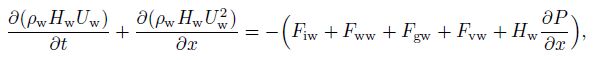
2.2.2 Momentum conservation equationsIn the multifluid model, the three phases exist in the pipe flow, resulting in three momentum equations. Despite the fact that hydrate will accumulate with time, the quantity is still small. In our study, we consider the hydrate coherent with water, which means that hydrates have the same velocity as water. Therefore, only two momentum equations (gas and water) are needed[14], i.e.,
 (10)
(10) 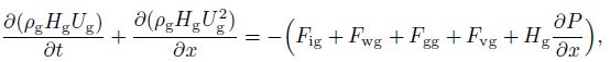 (11)
(11) where $F$ is the internal force between each phase (defined in Subsection 2.2.3). Solving Eqs.(10) and (11) with the volume fractions of water and gas, the velocities of water and gas $(U_{\rm g}$ and $U_{\rm w} )$ can be obtained. Then, using the condition of no slip between the hydrates and water, the velocity of the hydrates $(U_{\rm {hyd}} )$ can be obtained.
2.2.3 Internal forceThe internal force in the multiphase flow contains the drag force $(F_{{\rm i}k} )$, the frictional force $(F_{{\rm w}k})$, the body force $(F_{{\rm g}k})$, and the virtual force $(F_{{\rm v}k})$. Using the assumption of no slip between the hydrates and the water, the internal force of hydrates can be neglected[15].
The drag force depends on the pressure distribution acting on a material surface in the liquid-phase and the interfacial friction owing to the slip between the gas and the water. The drag force for gas $(F_{\rm {ig}})$ is defined by
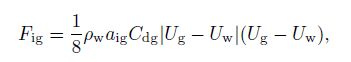 (12)
(12) where $a_{\rm {ig}} $ and $C_{\rm {dg}}$ denote the interfacial area concentration and the drag coefficient, respectively. These two parameters depend on the flow patterns of the gas-phase. The interfacial area concentration $(a_{\rm {ig}})$ is a parameter, which characterizes the structure of the flow and is based on the geometrical factors, the gas volume fraction, and the flow. According to Ishii et al.[16], the interfacial area per unit volume can be defined by
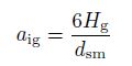 (13)
(13) in the bubble flow and
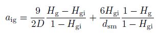 (14)
(14) in the slug and churn-turbulent flow, where $D$ is the pipe diameter, $d_{\rm {sm}} $ is the mean diameter of the small bubbles, and $H_{\rm g} $ is the average gas volume fraction. Kurul and Podowski[17] suggested that $H_{\rm {gi}}$ could be given by
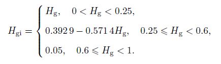 (15)
(15) Kocamustafaogullari et al.[18] gave the expression of the mean diameter of a small bubble as follows:
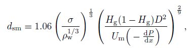 (16)
(16) where $\sigma $ is the surface tension. In this study, the pressure distribution is not considered. Therefore, $d_{\rm {sm}} $ can be regarded as zero. The drag coefficient $(C_{\rm {dg}})$ is also different for different flow patterns. Tomiyama et al.[19-20] proposed the drag coefficient in the bubble flow as follows:
 (17)
(17) 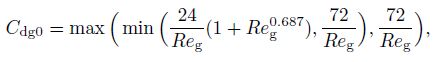 (18)
(18) where $Re_{\rm g}$ and $E_0$ denote the bubble Reynolds number and the Eotvos number, respectively, which are defined by
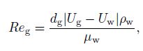 (19)
(19) 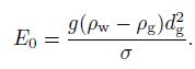 (20)
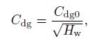
(20) Furthermore, the drag coefficient in the slug and churn flow can be defined with the gas volume fraction as follows:
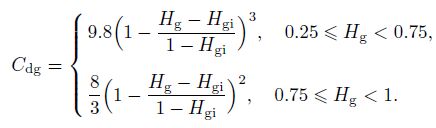 (21)
(21) The drag force for water $F_{\rm {iw}} $ is $-F_{\rm {ig}}$ because the internal force should be zero and the hydrate can be considered to be coherent with the water.
The frictional force $F_{{\rm w}k} $ is between the fluid and the pipe wall. The frictional force leads to the pressure drop. However, in this study, the pressure drop is neglected. Therefore, the frictional force is zero. In addition, the body force in a horizontal pipe is also zero. This is because that there is no gravity effect on the fluid along the pipeline. The virtual mass force appears when one phase is accelerating relative to the other. Lahey et al.[21] investigated the effects of the virtual mass on the accelerating of two-phase flows, and confirmed that the virtual mass force was very small and could be neglected.
In this study, the internal force that we are concerned is the drag force, which has been confirmed to be the most important force acting in the multiphase flow.
2.2.4 Energy balance equationThe energy balance equation is based on a homogenous model, where the fluid properties are the volume average of the independent phases[22]. In the equation, a source term $(S_{\rm e} )$ should be added to simulate the heat change accompanied with the phases change, i.e.,
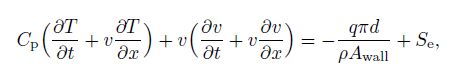 (22)
(22) where $C_{\rm p}$ is the mixture heat capacity defined with the phase fractions by
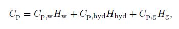 (23)
(23) $\frac{q\pi d}{\rho A_{\rm {wall}}}$ is a source term for the pipe wall heat transfer to the environment, $d$ denotes the pipe diameter, and $A_{\rm {wall}} $ is the surface area of the pipe. The wall heat flux $q$ can be calculated by a steady-state radial heat equation, considering the convection from the internal fluid to the pipe wall[23] as follows:
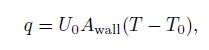 (24)
(24) where $U_0 $ is the overall heat transfer coefficient, $T$ is the fluid temperature, and $T_0 $ is the ambient temperature.
2.3 Transient hydrate kinetic modelThe hydrate formation rate can be written with the transient hydrate kinetic model[24] as follows:
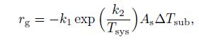 (25)
(25) where $r_{\rm g} $ is the rate of the gas consumption per unit volume during the hydrate formation, $k_1$ and $k_2 $ are the constants determined by a vast amount of experimental data, $A_{\rm s} $ is the surface between the water phase and the gas phase, $T_{\rm {sys}}$ is the fluid temperature, and $\Delta T_{\rm {sub}} $ is the subcooling temperature defined as the difference between the hydrate equilibrium temperature and the fluid temperature, i.e., $ \Delta T_{\rm {sub}} =T_{\rm {eq}} -T_{\rm {sys}}. $ $\Delta T_{\rm {sub}}>0$ means that a driving force exists and hydrates are produced in the flow.
The surface area $(A_{\rm s})$ is proposed as a function of the water phase volume fraction and the pipe radius $(r)$ in one-dimensional condition[25], i.e.,
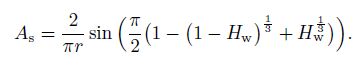 (26)
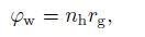
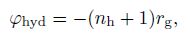
(26) With the transient hydrate kinetic model proposed above, the source term in the mass conservation equations and the energy balance equation can be defined due to the mass conservation of the chemical equation (27):
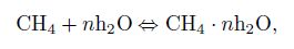 (27)
(27)  (28)
(28)  (29)
(29)  (30)
(30) where $n$ denote the hydrate number which is approximately 6[1], $n_{\rm h} $ is the hydration number determined by the chemical equation (27), and $\Delta h_{\rm {hyd}} $ is the heat of hydrate formation per unit volume needed.
3 Procedure of numerical calculationTo simulate the developed multifluid model, the finite difference method is used to simplify the mass conversation equation, the momentum equation, and the energy balance equation. The pipe segment is divided into equally spaced sections of the length ${\rm d}x$, and the nodes are numbered sequentially. Take Eq.(7) as an example to introduce the procedure.
 (31)
(31) where $n$ denotes the time step level of the temporal discretization, e.g., $n$ indicates the current time step and $n-1$ indicates the previous time step, $i$ denotes the node index for the spatial discretization, and ${\rm d}t$ is the time in each step. In all mass conversation equations, the momentum equations use a first-order backward difference scheme in the time scale and a third-order upwind scheme in the spatial scale. In addition, the first-order backward difference scheme is used in the energy balance equation.
In the simulation, the choices of ${\rm d}t$ and ${\rm d}x$ are not independent as ${\rm d}t/{\rm d}x$ appears in the difference equations. Generally, the ration of ${\rm d}t/{\rm d}x$ must obtain the Courant-Friedrichs-Lewy (CFL) criterion, i.e., ${\rm d}t/{\rm d}x<1$. Zerpa et al.[11] has found that when the CFL term is smaller than 0.15, the gas-liquid interface will stabilize to the stratified flow. In this study, the time step ${\rm d}t$ is chosen as 0.004 s for the multiphase flow model because of the small amount of the produced hydrate. Moreover, the gas density is regarded as a constant since no pressure drop is considered in this study and a periodic boundary condition is used as the boundary condition. The other parameters are as follows: the initial loop temperature is 302.7 K, the initial loop pressure is 6.9 MPa, the initial gas superficial velocity is 1.7 m$\cdot$s$^{-1}$, the initial water superficial velocity is 0.8 m$\cdot$s$^{-1}$, the pipe diameter is 0.097~2 m, the pipe length is 94 m, the pipe section length ${\rm d}x$ is 1 m, the transient kinetic model $k_1 $ is $7.354\times 10^{17}$ kg$\cdot$m$^{-2}\cdot$s$^{-1}\cdot$ K$^{-1}$, the transient kinetic model $k_2$ is $-13~600$ K, the water density is 1~000 kg$\cdot$m$^{-3}$, the hydrate density is 910 kg$\cdot$m$^{-3}$, the gas density is 55 kg$\cdot$m$^{-3}$, the water dynamic viscosity coefficient is $1.0\times 10^{-3}$ m$\cdot$s$^{-2}$, the surface tension is $7.2\times 10^{-2}$ N$\cdot$m$^{-2}$, and the heat transfer coefficient is $40$ w$\cdot$m$^{-2}\cdot$K$^{-1}$.
4 Results and analysesThe model proposed in Section 2 is derived from the multifluid model, and we will use it to predict the phase changes in the pipelines. Considering Ref.[11], we calculate the temperature of the fluid and the ambient temperature. The results are shown in Fig. 3. The results show that there are some differences between the simulation results and the experimental results. The main reason for these differences is that the provided ambient condition is different in different cases. In the experiments, the ambient temperature changes are not linear from 302.7 K (room temperature) to 273.15 K (freezing point). However, in the simulation, to simplify the process of cooling, we use a linear function (a decline of 0.000~4 K at every time step) to cool the temperature from 302.7 K to 272.15 K (below the freezing point). For the experimental data, the ambient temperature oscillates around 273.15 K. However, when it affects the fluid, the oscillation will be reduced. This phenomenon is reflected in the simulation as the steady fluid temperature for the ambient temperature stays at 272.15 K. From the figure, we can also see that the results from the simulation and the experiments are similar at the steady state.

|
| Fig. 3 Comparison of simulation results and experiment data[11] of fluid and ambient temperature |
|
|
The main purpose of the current work is to explore the hold-up changes of each phase. Figure 4 shows the results of the developed multifluid model. Figures 4(a), 4(b), and Figures 4(c) show the hold-up distributions along the pipeline at 6~000 s, 8~800 s, and 10~600 s, respectively. It is seen that, at 6~000 s, the fluid temperature is low enough to allow the formation of hydrates; at 8 800 s, the hold-up distribution begins to change as the hydrates accumulate over the period and act as a perturbation for the fluid. Finally, at 10~600 s, the fluid seems to be steady. At this time, the tendency shown at 8~800 s is exaggerated, and the hold-up difference between water and gas becomes larger. This phenomenon is caused by the hydrates produced between the water and the air, and indicates that a small amount of hydrates may cause a large effect on the hold-up changes.

|
| Fig. 4 Hold-up of each phase along pipeline length at different time |
|
|
In addition to the above analyses, it is also necessary to analyze the velocity field of each phase with the hold-up changes. From the momentum equations, we can see that, when the flow becomes steady, the force term is zero. In this study, only the drag force is considered, which means that the air velocity equals the water velocity. With the decrease in the steady velocity, the hold-up becomes steady.
5 ConclusionsThis work aims at exploring the hydrate effects in pipelines via a mechanical method. A simulation model is derived from a normal mutifluid model. Accounting for the multiple phases (water, hydrate, and gas), phase changes, and heat exchange across the flow, a one-dimensional model is used. In addition, a transient hydrate kinetics model is used to simulate the hydrate formation coupled with the mass conservation equations, and a mixture energy balance equation is used to predict the fluid temperature changes.
Comparing the simulation results with the experimental data reported in Ref.[11], because a little difference exits in the initial conditions, the results have some differences. However, when we consider the steady state, no difference exists between the experiments and the simulation. In addition to the temperature, the hold-up of water and gas appears to oscillate, and the maximum water hold-up ups to 0.7. This implies that slugs may occur at some points along the pipeline, and we should pay more attention to these areas because they may cause a reduction of transport efficiency and damage to the pipeline. Therefore, hydrates play an important role in water/gas system because the hydrate formation at the interfaces can interrupt the balance between the water and the gas.
In this study, only a one-dimensional model is completed. The one-dimensional model only can calculate the phase velocity and hold-up, while provides no information on the flow patterns. Actually, the flow pattern plays an important role in the simulation. For example, different flow patterns have different drag coefficients. In our simulation, the flow patterns are distinguished by the phase hold-up, but these results lack accuracy. In addition, turbulence is a complex flow, and must have feedback to the hydrate via the particle velocity and temperature. Therefore, there is still a lot to be done in the future, such as developing a three-dimensional model and adding a turbulence term to the one-dimensional model.
| [1] | Sloan, & E., D Clathrate Hydrates of Natural Gases (1998) |
| [2] | Burshears, M, ., O'Brien, T, ., and, Malone, & R A multi-phase, multi-dimensional, variable composition simulation of gas production from a conventional gas reservoir in contact with hydrates. SPE Journal, 1546, 449-453 (1986) |
| [3] | Makogon, & Y., F Hydrate of Hydrocarbons, PennWell Publishing Co. , Tulsa, Oklahoma (1997) |
| [4] | Clarke, M., and Bishnoi, & P., R Determination of the intrinsic rate constant of ethane gas hydrate decomposition. Chemical Engineering Science, 55, 4869-4883 doi:10.1016/S0009-2509(00)00137-8 (2000) |
| [5] | Clarke, M., and Bishnoi, & P., R Determination of the activation energy and intrinsic rate constant of methane gas hydrate decomposition. The Canadian Journal of Chemical Engineering, 79, 143-147 doi:10.1002/cjce.v79:1 (2001) |
| [6] | K, im, H., C., Bishnoi, P., R., Heidemann, R., A., and, Rizvi, & S., S. H Kinetics of methane hydrate decomposition. Chemical Engineering Science, 42, 1645-1653 doi:10.1016/0009-2509(87)80169-0 (1987) |
| [7] | S, un, X., F. and Kishore, & K., M Kinetic simulation of methane hydrate formation and dissociation in porous media. Chemical Engineering Science, 61, 3476-3495 doi:10.1016/j.ces.2005.12.017 (2006) |
| [8] | Carroll, & J Nature Gas Hydrates:A Guide for Engineers. Gulf Publishing (2002) |
| [9] | Cr, ee, L., J. L. and Subramanian, & S New methods for managing hydrates in deepwater tiebacks. Proceedings of the Offshore Technology Conference, Huston, Texas (2011) |
| [10] | Denielson, & T., J A simple model for hydrodynamic slug flow. Proceedings of the Offshore Technology Conference, Huston, Texas (2011) |
| [11] | Zerpa, L., E., Ishan, R, ., Am, an, Z., M., Danielson, T., J., K, oh, C., A., Sloan, E., D., and, Sum, & A., K Multiphase flow modeling of gas hydrates with a simple hydrodynamic slug flow model. Chemical Engineering Science, 99, 298-304 doi:10.1016/j.ces.2013.06.016 (2013) |
| [12] | Turner, D., J. Clathrate Hydrate Formation in Water-in-Oil Dispersion, & P, h D. dissertation, Colorado School of Mines, Colorado (2005) |
| [13] | Yu, an, Y., R., Zh, ao, W., D., Cheng, A., J., and, Han, & Y., J Simulation and application of threedimensional migration-accumulation of oil resources. Applied Mathematics and Mechanics (English Edition), 20(9), 999-1000 (1999) |
| [14] | Natsuo, H, ., Hitoshi, F, ., and, Makoto, & I Theoretical analysis of flow characteristics of multiphase mixtures in a vertical pipe. International Journal of Multiphase Flow, 24, 539-561 doi:10.1016/S0301-9322(97)00074-8 (1998) |
| [15] | Chaudhary, R., C. and Abhay, & K., J Effects of chemic reactions on MHD micropolar fluid flow past a vertical plate in slip-flow regime. Applied Mathematics and Mechanics (English Edition), 29(9), 1179-1194 doi:10.1007/s10483-008-0907-x (2008) |
| [16] | Ishii, M, ., Mishima, K, ., Kataoka, I, ., and, Kocamustafaogullarim, & G., Two-fluid model and importance of the interfacial area in two-phase flow analysis Proceedings of 9th U.S. National Congress of Applied Mechanics, Ithaca, New York, 73-80 (1982) |
| [17] | Kurul, N, ., and, Podowski, & M., Z On the modelling of multidimensional effects in boiling channels. Proceedings of the 27th National Heat Transfer Conference, Minneapolis (1991) |
| [18] | Kocamustafaogullari, G, ., Huang, W., D., and, Razi, & J Measurement and modelling of average void fraction, bubble size and interfacial area. Nuclear Engineering and Design, 48, 437-453 (1994) |
| [19] | Tomiyama, A, ., Kataoka, I, ., and, Sakaguchi, & T Drag coefficient of bubbles-1st report, drag coefficient of a single bubble in a stagnant liquid. Transactions of the Japan Society of Mechanical Engineers, Part B, 61, 2357-2364 doi:10.1299/kikaib.61.2357 (1995) |
| [20] | Tomiyama, A, ., Kataoka, I, ., Fukuda, T, ., and, Sakaguchi, & T Drag coefficient of bubbles-2nd report, drag coefficient of a swarm of bubbles in and its applicability to transient flow. Transactions of the Japan Society of Mechanical Engineers, Part C, 61, 2810-2817 doi:10.1299/kikaib.61.2810 (1995) |
| [21] | Lahey, R., T., Cheng, L., Y., Dr, ew, D., A., and, Flaherty, & J., E The effect of virtual mass on the numerical stability of accelerating two-phase flows. International Journal of Multiphase Flow, 6, 281-294 doi:10.1016/0301-9322(80)90021-X (1980) |
| [22] | Cazarez-Candia, O., and Vasquez-Cruz, & M., A Prediction of pressure, temperature and velocity distribution of two-phase flow in oil wells. Journal of Petroleum Science and Engineering, 46, 195-208 doi:10.1016/j.petrol.2004.11.003 (2005) |
| [23] | B, ai, Y., and Bai, & Q Heat transfer and thermal insulation. Subsea Piplelines and Risers-Part Ⅲ:Flow Assurance, Elsevier, 317-356 (2005) |
| [24] | Boxall, J, ., Davies, S, ., K, oh, C., A., and, Sloan, & E., D Predicting when and where hydrate plugs form in oil-dominated flowlines. SPE Projects Facilities and Construction, 4, 80-86 doi:10.2118/129538-PA (2009) |
| [25] | Biberg, & D An explicit approximation for the wetted angle in two-phase stratified pipe flow. The Canadian Journal of Chemical Engineering, 77, 1221-1224 doi:10.1002/cjce.v77:6 (1999) |