 2016, Vol. 37
Shanghai University
Article Information
- huiGAO Ying, yingMENG Xiang, shaoLU Qi
- Border collision bifurcations in 3D piecewise smooth chaotic circuit
- Applied Mathematics and Mechanics (English Edition), 2016, 37(9): 1239-1250.
- http://dx.doi.org/10.1007/s10483-016-2129-6
Article History
- Received Dec. 25, 2015
- Revised Mar. 11, 2016


2. Department of Biology, University of Maryland, College Park, MD 20742, U. S. A;
3. School of Aeronautic Science and Engineering, Beihang University, Beijing 100191, China
Bifurcations and chaos in smooth dynamical systems have been well developed in both theoretical and applied researches. However,there still exist some kinds of piecewise smooth systems in the fields of science and engineering. The studies of bifurcations and chaos in them have been concerned in recent years [1-14]. Piecewise smooth systems,even the simplest linear piecewise systems,may exhibit extremely complex dynamics,and are worthy of being studied. The variation of time can be either continuous or discrete. The state space of a piecewise smooth system is composed of several regions,in which the system is controlled by different smooth functions. On the boundaries of these regions,the control functions are discontinuous or non-smooth. It is better to analyze the dynamical behaviors of the piecewise smooth systems in both theoretical ways and numerical ways due to the difficulties.
The results show that there exist a kind of peculiar bifurcations when the orbit of the piecewise smooth system has the tangency with the boundary. Nusse and Yorke[15-16] coined the term “border collision bifurcation” to describe this class of nonlinear phenomena,for which the term ”C-bifurcation” was used in some Russian literatures instead. The dynamical behaviors may change acutely at this time,e.g.,periodic orbits may transit to chaos orbits directly. This kind of bifurcations can occur only in non-smooth systems instead of smooth systems. Similar to the bifurcations in smooth systems,there are many kinds of border collision bifurcations such as non-smooth fold bifurcations and non-smooth flip bifurcations.
For the piecewise smooth systems with continuous time,di Bernardo et al.[17] obtained the Poincaré map with the piecewise form by locally linearizing the periodic solution near the border collision bifurcation,and gave the classification method of the border collision bifurcation. Without constructing the Poincaré map,Leine and Nijmeijer[18] obtained the generalized Jacobian matrix by using the generalized Clarke derivative,and gave some classification methods of border collision bifurcations by means of the eigenvalues of this matrix. The eigenvalues of the generalized Jacobian matrix were set-valued,and formed a one-dimensional (1D) path in the complex plane. The eigenvalue may cross the imaginary axis either continuously or through a jump under the variations of the parameters. Especially,non-smooth continuous systems can also exhibit equilibrium bifurcations,for which a 1D path of eigenvalues may cross the imaginary axis for the multiple time. Multiple crossing bifurcations are much more complex than single crossing bifurcations. They do not have a smooth counterpart. As a whole,border collision bifurcations are a new kind of bifurcations in piecewise smooth systems,and are worthy of understanding the boundary effects in non-smooth dynamics.
The Rössler attractor[19] is a famous chaotic system with single quadratic nonlinearity. But the Rössler system is relatively complicated[20],and researchers were prompted to search similar examples[21],in which the quadratic nonlinearity was replaced by |x| or other elementary piecewise linear functions. Sprott[22] found chaos in the electrical circuit 

This paper is organized as follows. In Section 2,we show the model and the existence of the equilibrium points. The stability of the two equilibrium points (
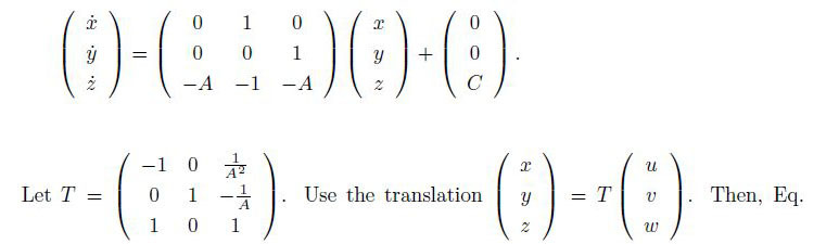
We consider the following circuit proposed by Sprott[22]:

Let x=y and y=z. Then,Eq.(1) can be transformed to the following three-dimensional (3D) piecewise smooth system:

When x > 0,Eq.(2) becomes

where

It is easy to see that,when 
When x <0,Eq.(2) becomes

where

When BC >0,
Through the above analysis,we can see that the two equilibrium points 


Proposition 1 The equilibrium point


Proof Denote

Then,the discriminant of Eq.(5) is

Since Δ<0 for 0<A<

where

It is easy to see that ζ >0 for 0 <A<
Let

Then,

Then,Re

The positive root of f(x)=0 is

Therefore,

Therefore,x1 >x2.
The graphs of f(x) and g(x) are shown in Fig. 1.

|
| Fig. 1 Graphs of f(x) and g(x) for A=0.6 |
|
|
The equilibrium point 

and

Therefore,ζ3 >x13,which leads to ζ>x1. Thus,

Proposition 2 The equilibrium point 

Proof Denote

Then,the discriminant of Eq.(6) is

It is easy to obtain that Δ <0 for 0<A

where

Since

we have η >0.
The equilibrium point 

In the following,we will show that

In fact,from Eq.(7),it can be obtained that 

Let

Then,


Moreover,


 (10)
(10) From Eqs.(9) and (10),we have

Then,from Eq.(8),we have 

and 
Proposition 3 The equilibrium point


Proof From the proof of Proposition 2,we can see that the equilibrium point 


Since (2A2-9)A<0 holds for 

Denote

The discriminant is

where Δ <0 when 


which has the following three eigenvalues:

where

When 

When 

In order to guarantee that q≤1,we require that A≤ B. The above results show that the eigenvalues cross the imaginary axis twice. Then,we have the following theorem.
Theorem 1 The multiple crossing of the eigenvalues of J(O) occurs at C=0 for A≤ B and
It should be noticed that bifurcations may be accompanied with the multiple crossing of the eigenvalues. Referring to Ref.[22],an example is taken for the parameter values A=0.6 and B=1. In Fig. 2,we depict the characteristic curves of J(O),where q is a path parameter. The eigenvalues γ1,γ2,and γ3 are set-valued,and form a path in the complex plane. γ1 crosses the origin at 


|
| Fig. 2 Paths of eigenvalues of J(O) for A=0.6 and B=1 |
|
|

|
Fig. 3 Non-smooth fold bifurcation,where  |
|
|

|
| Fig. 4 Periodic orbit Γ in system (2),where A=0.6, B=1,and C=0.5,along with an orbit with initial value (0.48,0, 0) |
|
|
Here,we present some theoretical results about the border collision bifurcations of Eq.(2). Through the above analysis in Section 3,we have the following Theorems 2 and 3.
Theorem 2 A non-smooth fold bifurcation can occur at O(0,0,0) for 


This situation is a part of the multiple crossing bifurcation and cannot occur in smooth fold bifurcations.
As an example,the bifurcation diagram is plotted in Fig. 3 for A=0.6 and B=1.
Theorem 3 Non-smooth fold bifurcation can occur at O(0,0,0) for


This situation is similar to the exchange of stability in smooth fold bifurcations.
The bifurcation diagram is plotted in Fig. 5 for A=1.2 and B=1,which is not a multiple crossing bifurcation

|
Fig. 5 Non-smooth fold bifurcation,where   |
|
|
The non-smooth Hopf bifurcation of Eq.(2) can be verified by numerical simulations,while is hard to be proceeded by theoretical analyses. However,for the special case with A=B,we have the following theorem.
Theorem 4 There exists a non-smooth Hopf bifurcation at O(0,0,0) for A=B.
Proof When A=B,there are two unstable equilibrium points 

 (11)
(11) becomes
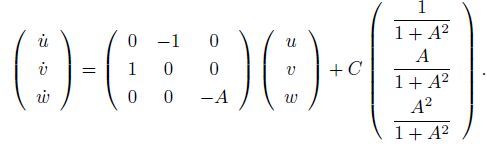 (12)
(12) x≥ 0 means that 
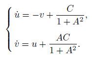 (13)
(13) After calculations,we have the first integration of Eq.(13) as follows:

i.e.,

where C1 is an arbitrary constant. Now,we can see that the solution of Eq.(13) corresponds to a circle on the (u,v)-plane.
From Eq.(12),we have
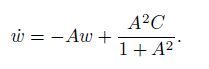 (14)
(14) The solution of Eq.(14) is given by

where C2 is an arbitrary constant,and
 (15)
(15) Now,we get the solution of Eq.(12) as follows:
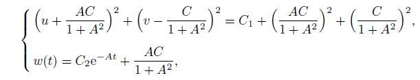 (16)
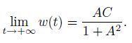
(16) which tends to the periodic solution
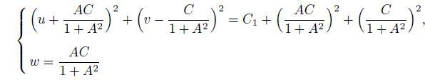 (17)
(17) when t→ +∞. From Eq.(16),we have

and

Therefore,under the condition
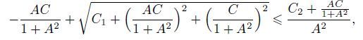 (18)
(18) we have

In fact,in order to guarantee that x(t)≥0 in Eq.(11),we can choose the proper value of C1 and

such that Eq.(18) holds. Together with Eq.(15),we can conclude that the periodic solution (17) is locally asymptotically stable. The center of the above circle is

It is easy to verify that it corresponds to the point 

Let C→ 0 in Eq.(18). Then,we can get

Since 
In a word,a non-smooth Hopf bifurcation occurs. The equilibrium point 

|
| Fig. 6 Periodic orbit in system (11) for A=1 and C=0.5, along with an orbit with initial value (0.48,0,0) |
|
|
Theorems 2 and 4 show that a multiple crossing bifurcation occurs at O(0,0,0) for A=B,which is the composite of a non-smooth fold bifurcation and a non-smooth Hopf bifurcation as seen in Fig. 7. This is a very interesting phenomenon. In usual smooth Hopf bifurcations,the equilibrium points locate at both sides of the bifurcation point,and there exists the exchange of stability between the equilibrium points. Nevertheless,here,the two equilibrium points are both unstable,and are located at the same side of the bifurcation point,without the exchange of stability between them.

|
| Fig. 7 Multiple crossing bifurcation at O(0,0,0) of system (2) for A=B=1,which is composite of non-smooth fold bifurcation and non-smooth Hopf bifurcation |
|
|
The border collision bifurcations in a 3D piecewise smooth chaotic electrical circuit simplified from the Rössler attractor are discussed.
It is found that there are three types of such bifurcations. When A≤ B,the two equilibrium points 


The multiple crossing bifurcation is also studied for C=0. The paths of the eigenvalues of the generalized Jacobian matrix and bifurcation diagrams are plotted to verify the analysis. It can be thought as the composite of a non-smooth fold bifurcation and a non-smooth Hopf bifurcation with some features different from those of usual smooth bifurcations.
| [1] | Di, Bernardo, M, ., Bu, dd, C., J., and, Champneys, & A., R Normal form maps for grazing bifurcations in n-dimensional piecewise smooth dynamical systems. Physica D, 160, 222-254 (2001) |
| [2] | Halse, C, ., Homer, M, ., and, di Bernardo, & M C-bifurcations and period-adding in one-dimensional piecewise smooth maps. Chaos, Solitons & Fractals, 18, 953-976 (2003) |
| [3] | Kumar, A, ., Banerjee, S, ., and, Lathrop, & D., P Dynamics of a piecewise smooth map with sigularity. Physics Letters A, 337, 87-92 (2005) |
| [4] | Sushko, I, ., Agliari, A, ., and, Gardini, & L Bifurcation structure of parameter plane for a family of unimodal piecewise smooth maps:border collision bifurcation curves. Chaos, Solitons & Fractals, 29, 756-770 (2006) |
| [5] | Zhusubaliyev, Z. T. and Mosekilde, E. Bifurcation and Chaos in Piecewise-Smooth Dynamical Systems, World Scientific, Singapore ,2003 |
| [6] | Banerjee, S., and Grebogi, & C Border collision bifurcations in two-dimensional piece-wise smooth maps. Physical Review E, 59, 4052-4061 (1999) |
| [7] | Banerjee, S, ., Karthik, M., S., Yu, an, G., H., and, Yorke, & J., A Bifurcations in one-dimensional piecewise smooth maps-theory and applications in switching circuits. IEEE Transactions on Circuits and Systems-I, 47, 389-394 (2000) |
| [8] | Banerjee, S, ., Ranjan, P, ., and, Grebogi, & C Bifurcations in two-dimensional piece-wise smooth mapstheory and applications in switching circuits. IEEE Transactions on Circuits and Systems-I, 47, 633-643 (2000) |
| [9] | Q, in, Z., Y., Ya, ng, J., C., Banerjee, S, ., and, Jiang, & G., R Border-collision bifurcations in a generalized piecewise linear-power map. Discrete and Continuous Dynamical System-Series B, 16, 547-567 (2011) |
| [10] | Prunaret, D., F., Chargé, P, ., and, Gardini, & L Border collision bifurcations and chaotic sets in a two-dimensional piecewise linear map. Communications in Nonlinear Science and Numerical Simulation, 16, 916-927 (2011) |
| [11] | Tramontana, F., and Gardini, & L Border collision bifurcations in discontinuous one-dimensional linear-hyperbolic maps. Communications in Nonlinear Science and Numerical Simulation, 16, 1414-1423 (2011) |
| [12] | Gardini, L, ., Tramontana, F, ., and, Banerjee, & S Bifurcation analysis of an inductorless chaos generator using 1D piecewise smooth map. Mathematics and Computers in Simulation, 95, 137-145 (2014) |
| [13] | F, u, S., H., L, u, Q., S., and, Meng, & X., Y New discontinuity-induced bifurcations in Chua's circuit. International Journal of Bifurcation and Chaos, 25, 25, 1550090 (2015) |
| [14] | F, u, S., H., Me, ng, X., Y., and, Lu, & Q., S Stability and boundary equilibrium bifurcations of modified Chua's circuit with smooth degree of 3. Applied Mathematics and Mechanics (English Edition), 36(12), 1639-1650 (2015) |
| [15] | Nusse, H., E. and Yorke, & J., A Border-collision bifurcations including "period two to period three" for piecewise smooth maps. Physica D, 57, 39-57 (1992) |
| [16] | Nusse, H., E. and Yorke, & J., A Border-collision bifurcations for piecewise smooth one dimensional maps. International Journal of Bifurcation and Chaos, 5, 189-207 (1995) |
| [17] | Di, Bernardo, M, .Feigin, M., I., Hogan, S., J., and, Homer, & M., E Local analysis of C-bifurcation in n-dimensional piecewise smooth dynamical systems. Chaos, Solitons & Fractals, 10, 1881-1908 (1999) |
| [18] | Leine, R. I. and Nijmeijer, H. Dynamics and bifurcations of non-smooth mechanical systems. Lecture Notes in Applied and Computational Mechanics, Springer-Verlag, Berlin ,2004 |
| [19] | Rössler, & O., E An equation for continuous chaos. Physics Letters A, 57, 397-398 (1976) |
| [20] | Li, nz, & S., J Nonlinear dynamical models and jerky motion. American Journal of Physics, 65, 523-525 (1997) |
| [21] | Sprott, & J., C Simple chaotic systems and circuits. American Journal of Physics, 68, 758-763 (2000) |
| [22] | Sprott, & J., C A new class of chaotic circuit. Physics Letters A, 266, 19-23 (2000) |