 2016, Vol. 37
Shanghai University
Article Information
- WANG Dan, CHEN Yushu, WIERCIGROCH M., CAO Qingjie
- Bifurcation and dynamic response analysis of rotating blade excited by upstream vortices
- Applied Mathematics and Mechanics (English Edition), 2016, 37(9): 1251-1274.
- http://dx.doi.org/10.1007/s10483-016-2128-6
Article History
- Received Dec. 23, 2015
- Revised Apr. 25, 2016


2. Centre for Applied Dynamics Research, School of Engineering, University of Aberdeen, King's College, Aberdeen AB24 3 UE, Scotland, U. K
Vortex shedding is often observed in engineering,such as circular cylinders in cross-flow[1],oscillating airfoils and turbomachine blades[2],and micro air vehicles[3]. Lai and Platzer[2] studied different vortex patterns shedding from the trailing edge of an NACA 0012 airfoil,and found that the vortex patterns oscillated sinusoidally in the plunge were captured in water tunnel tests with a Reynolds number range from 500 to 21 000 based on the airfoil chord. Gostelow et al.[4] showed a strong similarity between the vortex wakes shed from cylinders and airfoils with the sinusoidal plunge motion in the low-speed flow and the wakes shed from a turbine nozzle cascade in the transonic flow,and presented the thermo-acoustic effect associated with the vortex shedding in the rotating machines. Lawaczek and Heinemann[5-6] found a turbine blade with a blunt trailing edge to shed a von Kármán vortex street. Aeroelastic problems may occur easily in operating the conditions owing to the vortex shedding,such as the flutter for the aircraft wings,helicopter,and turbine blades.
For a fluid-structure interaction (FSI) problem,the vortex-induced vibration is difficult in modelling the coupled loads. Because both experimental[7] and numerical[8-11] approaches are expensive to obtain robust results,simplified models were developed to reveal the nonlinear effects of the system parameters on the dynamic responses of the system. Generally,turbine blades are simplified as the elastic clamped-free beams in both experimental[12] and numerical analyses[13-16]. Cao et al.[17] and Chu et al.[18] analyzed the two-dimensional friction contact problem and impact vibration characteristics of a rotational blade in the centrifugal force field,and simplified the blade as a continuous cantilever.
The van der Pol model for the FSI problem have been widely studied. The results show that the self-excited oscillation for the structure owns to the characteristic of the time-varying[19-21]. Lee et al.[22] used a van der Pol oscillation to model an aeroelastic system possessing limit cycle oscillations. Specifically,Hartlen and Currie[23] introduced a van der Pol-based model,which captured many of the features seen in experimental results. Skop and Griffin[24] subsequently modified and improved the van der Pol-based model. The vortex-induced vibrations for a cylinder[25],an offshore riser[26],and a turbine blade[27] have also been analyzed,where the time-varying characteristics of the vortices are modelled by the van der Pol oscillation,and the effects of the structural motion on the fluid are studied. Barron and Sen[15] added a van der Pol damping term to the equations of four coupled elastic beams to represent the self-excitation and fluid-structure interaction of the system. Barron[16] simulated the FSI problem for turbine blades by adding a van der Pol self-exciting term to a single partial differential equation of a linear beam. Wang et al.[28] used the van der Pol oscillator to simulate the time-varying characteristics of the lift coefficient for the fluid-structure interactions of turbine blades.
Moreover,it has been demonstrated that the vortex shedding from oscillating airfoils and cylinders can be significantly affected by the body oscillation[1, 25-26, 29-33]. Therefore,to analyze the vibrations of the vortices further,it is necessary to consider the action of the structural motion on the fluid.
The motivation of this paper is to investigate the dynamic response and bifurcation characteristics for the vortex-induced vibrations of a rotating blades. The blade is modelled as a cantilever beam,while a van der Pol equation is used to mimic the time-varying characteristics for the vortices. The reaction of the structural motion on the fluid is considered and represented by a linear inertial coupling. The 1:1 internal resonance analysis is carried out with the multiple scale method. The two-parameter bifurcation diagram is derived by the singularity theory,and the frequency-response curves in different parameter regions are obtained. The time histories,phase portraits,and Lyapunov exponents are calculated by the Runge-Kutta method for the original system to verify the validity of the multiple scale method.
2 Mathematical modelling 2.1 Cantilever beam model for bladeIn engineering practice,the rotating Euler-Bernoulli beam[34-35] is often used to analyze the dynamic characteristics of engineering systems,such as turbomachinery,wind turbines,robotic manipulators,and rotorcraft blades. To investigate the interaction mechanism of the structure and fluid,the blade is assumed to be a continuous uniform straight cantilever beam based on the Euler-Bernoulli formulation in the centrifugal force field (see Fig. 1).

|
| Fig. 1 Sketches of blades excited by upstream vortices |
|
|
The transverse motion of the beam will be mainly studied,and the effects of the shear deformation and rotatory inertia are neglected. özgür and Gökhan[35] studied the in-plane vibrations of a rotating Euler-Bernoulli beam with the Coriolis force,and revealed that all the coefficients related to the Coriolis force would vanish during the reduction processing,where a single degree-of-freedom model for the ith mode vibration was extracted by the Galerkin method. Therefore,there is no Coriolis term in the single degree-of-freedom equation.Xu et al.[36] demonstrated that the Coriolis force had no influence on the axial and torsional vibrations of the rotating blades,and the effect on the tangential vibration was very small and could be neglected. Therefore,the effect of the Coriolis force on the rotating blade is neglected in this study.
The transverse displacement of the cantilever beam is assumed as w(x,t),and the equation of the blade motion can be derived by considering the equilibrium of the forces and moments acting on the differential segment of the blade with the length of dx (see Fig. 2). For more details,please refer to Ref.[17].

|
| Fig. 2 Free-body diagram of differential segment |
|
|
The first dynamic equilibrium relationship with respect to the transverse displacement w(x,t) can be obtained by summing all the forces in the transverse direction for the segment,i.e.,

where m=(p+pf)A is the total mass consisting of the structure and the added mass induced by the fluid,p and pf are the densities of the structure and air flow,respectively,and A is the area of the cross-section for the cantilever beam. p and A are constants according to the beam assumption. Q is the shear force acting on the cross-section of the blade. c is the viscous damping coefficient. f is the axial load expressed as follows (see Fig. 1(b)):

where L is the length of the blade,and Ω is the rotating speed of the blade. Ff is the fluid force acting on the blade induced by the vortices,i.e.,

where CL is the lift coefficient representing the time-varying characteristics of the vortices,and U is the total velocity defined by 
Neglecting the shear deformation and the rotation of the cross-section according to the beam assumption,when the condition of moment equilibrium is satisfied,we can introduce the basic moment-curvature relationship as follows:

where M is the moment acting on the cross-section of the beam,and EI is the flexural rigidity of the structure. With Eq.(2),we can simplify Eq.(1) as follows:

Substitute the following non-dimensional variables:

into Eq.(3). Then,we have

The boundary conditions of the cantilever beam should meet the following conditions:
(i) When z=0,the displacement and rotation of the beam should be equal to zero,i.e.,

(ii) When z=1,the moment and shear force should be equal to zero,i.e.,
2.2 Van der Pol oscillator
The van der Pol oscillator is often used to model the time-varying and self-sustained characteristics of the flow in the analytical/experimental research of vortex-induced vibrations. The lift coefficient can represent the flow characteristics[25-26],which can affect the lift force and then the structural vibrations. Herein,the van der Pol oscillator is introduced to simulate the time-varying characteristics of the lift coefficient,i.e.,

where q(z,t)=2 CL/CL0,in which CL0 is the reference lift coefficient,wf=2π StV/D0 is the shedding frequency of the vortex,St is the Strouhal number,and λ is the van der Pol damping coefficient. Moreover,the action of the structural vibration on the fluid motion FS is considered to be outlined in the introduction. It has been shown in Refs.[25] and [26] that the inertial coupling is the ideal form to describe the reaction of the blades to the flows. Therefore,the linear inertial coupling is studied,and the force FS induced by the structural motion can be assumed as follows:

where N~ is the linear coupling parameter.
To analyze in the same time scale,let T =Ω t. Then,Eq.(6) becomes

Therefore,the coupled equations (5) and (7) model the interactions of the blade and vortices.
2.3 Reduced model with Galerkin discretizationAn arbitrary oscillation of the structure v(z,T ) can be accurately described with a sum of all of its modal responses,which can be mathematically expressed with a Taylor series composed of the individual modal components[37] as follows:

where v~i (z) and vi (T) (i=1,2,...) represent the mode shapes and the modal coordinates of the beam,respectively. When the shapes of the deformation are known,the modal coordinates vi (T) (i=1,2,...) define how the amplitudes of the associated deformations v~i (z)(i=1,2,...) change with time. Thus,the continuous system can be discretized by defining it on the modal subspaces.
For the approximate solution,the orthonormal sets of the eigen amplitude functions for a cantilever beam as the modal functions for the blade are introduced,i.e.,

where βi(i=1,2,...) are the roots of the transcendental equation

which is derived from the boundary conditions of the cantilever beam.
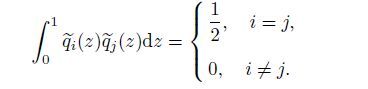
Herein,the cross-section of the beam is assumed to be uniform. Therefore,the orthogonality of different modal functions can be written as follows:
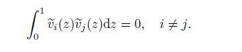 (10)
(10) It means that the spatial distributions of the structure are perpendicular to each other in the modal space if they are not of the same order.
When the modal functions are in the same order,the integral can be calculated as follows:
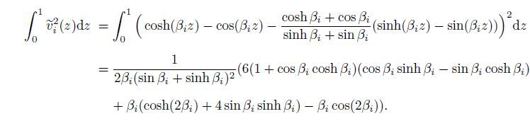 (11)
(11) It can be seen from Eq.(11) that the value of the integral can be determined by the corresponding coefficient βi.
The span-wise distribution of the shedding variable has been widely studied[38-43],in which the spatial component of q(z,T ) is described with the shape of the respective normal mode and separated from the temporal part of the response. Hence,the form of the solution q(z,T ) can be assumed to be expressed with a Taylor series of modal components as analyzed in Refs.[39]-[43],i.e.,
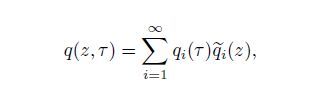 (12)
(12) where the relations between the mode-shapes 
The modal functions for the van der Pol oscillator are introduced according to Ref.[43],i.e.,
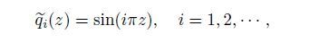 (13)
(13) which satisfy the following orthogonality condition:
 (14)
(14) With the relation

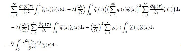
substituting Eq.(8) into Eq.(5) and orthogonalizing the latter with respect to the set v~j (z),we have
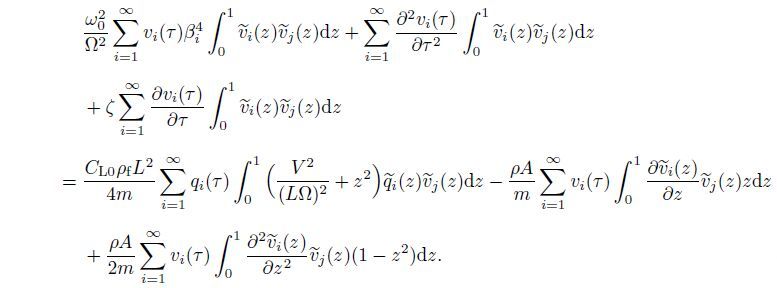 (15)
(15) Because the fluid-structure interaction problem considered in this study is an ideal one,the fluid force can induce the structural oscillation in only one mode. Therefore,the van der Pol oscillator can be expected to have the same and single modal distribution in the space,and the first modal approximations of the cantilever beam and the van der Pol oscillator can be investigated.
The first mode equation of the structure can be derived from Eq.(15) when i=j=1,i.e.,
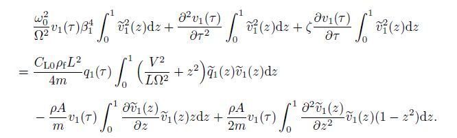 (16)
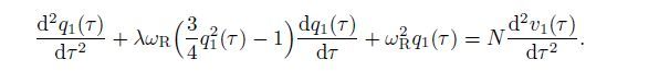
(16) Thus,the first-order equation for the cantilever beam can be simplified as follows:
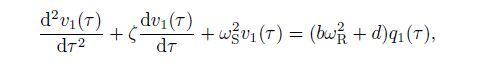 (17)
(17) where wR =w f/Ω is the non-dimensional frequency of the fluid,


The values of the above definite integrals can be obtained when the coefficient β1 is determined.
Similarly,substituting Eq.(12) into Eq.(7) and orthogonalizing the obtained results with respect to q~j (z),we have
 (18)
(18) Furthermore,it can be rewritten as follows:
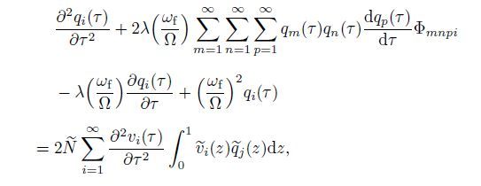 (19)
(19) where
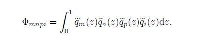 (20)
(20) When m=n=p=i=1,Eq.(20) can be simplified as follows:
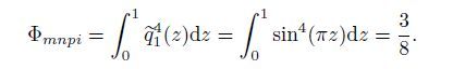 (21)
(21) When i=j=1,we introduce

as the inertia coupling parameter,which denotes the action for the first mode motion of the structure on the first mode motion of the van der Pol oscillator. Thus,the first mode motion of the van der Pol oscillator can be derived as follows:
 (22)
(22) Equations (17) and (22) model the interactions between the structural vibration and the van der Pol oscillation,and will be investigated in the following sections.
3 Bifurcation analysis 3.1 1:1 internal resonance analysis with multiple scale methodWhen the resonance occurs[44-45],such as the primary resonance,the internal resonance,and the superharmonic/subharmnic resonance,the nonlinear systems display the rich dynamic characteristics. The multiple scale method is a good way for understanding the qualitative characteristics of the system presenting the internal resonance[46-48]. The phenomenon of lock-in or synchronization is often analyzed in the vortex-induced vibration for the long cylinders (e.g.,the offshore risers),which means that the vortex shedding frequency fV tends to the natural frequency of the structure fS [29]. Similarly,the phenomenon for the frequency approximation can also be encountered in the coupled system proposed in this paper. For Eqs. (17) and (22),the non-dimensional frequencies wS and wR of the first-order coupled system (see Fig. 3) are approximate to each other around the rotating speed Ω≈ 450 rad·s−1.

|
| Fig. 3 Non-dimensional frequencies wS and wR varying with rotating speed Ω |
|
|
Hence,the 1:1 internal resonance of the coupled system is interesting,and will be investigated by the multiple scale method. The relation between the non-dimensional frequencies wS and wR can be written as follows:

where σ is the detuning parameter. Introducing the scaling parameters

into Eqs.(17) and (22),we have
 (23)
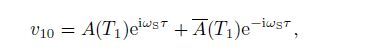
(23) Assume the approximate form of the solutions as follows:
 (24)
(24) Then,substituting Eq.(24) into Eq.(23) and equating the coefficient of like powers of ε,we have the results of the order ε 0 as follows:
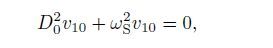 (25)
(25) 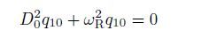 (26)
(26) and the order ε ^1 as follows:
 (27)
(27) 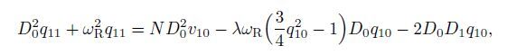 (28)
(28) where

and 
 (29)
(29)  (30)
(30) Substitute Eqs.(29) and (30) into Eqs.(27) and (28). Consider the internal resonance condition. Then,we have
 (31)
(31) 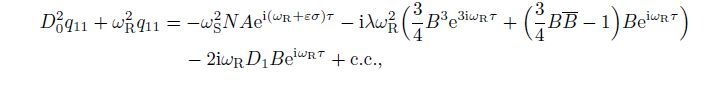 (32)
(32) where c.c. stands for the complex conjugate of the proceeding terms.
The solvable conditions of Eqs.(31) and (32) are derived by equating the coefficients of the secular terms to be zero,i.e.,
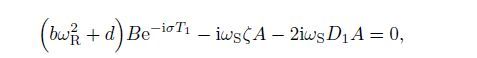 (33)
(33) 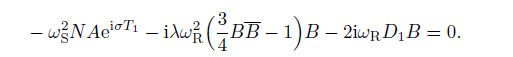 (34)
(34) The derivatives of the amplitudes A and B with respect to T1 can be obtained by Eqs.(33) and (34) as follows:
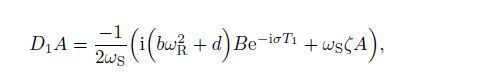 (35)
(35) 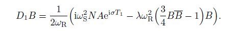 (36)
(36) The functions A and B can be expressed in the polar coordinates as follows:
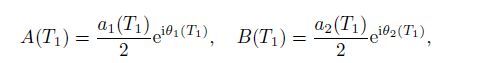 (37)
(37) where aj and θj(j=1,2) are the amplitudes and phase angles,respectively. Substituting Eq.(37) into Eqs.(35) and (36) yields the following first-order differential equations after separating the real and imaginary parts:
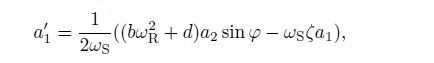 (38)
(38) 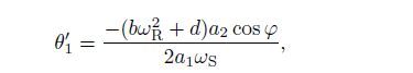 (39)
(39) 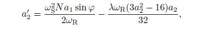 (40)
(40) 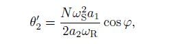 (41)
(41) where (′) denotes the derivatives with respect to T1,and φ = θ 2 - σ T1 - θ 1. The derivative of φ with respect to T1 can be obtained by eliminating θ1 and θ_2 from Eqs.(39) and (41) as follows:
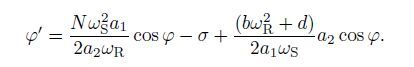 (42)
(42) The equilibrium solutions of Eqs.(38),(40),and (42) correspond to the periodic motion of the coupled system. To obtain the equilibrium solutions,a′j(j=1,2) and φ′ in Eqs.(38),(40),and (42) are assumed to be equal to zero. Then,we can obtain the frequency-response equations as follows:
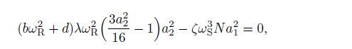 (43)
(43) 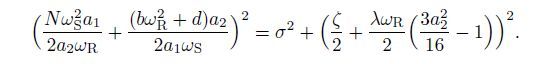 (44)
(44) Equations (43) and (44) can reveal the effects of the system parameters on the responses.
3.2 Singularity analysis for steady-state responsesThe structural motion and the van der Pol damping have important effects on the vibration of the fluid. Then,the fluid motion in turn can affect the structural vibration. To investigate the bifurcation characteristics of the coupled system in a wider parameter space,an engineering unfolding analysis is carried out (see Refs.[49]-[51] for the details). Equations (43) and (44) can be rewritten as follows:
 (45)
(45) 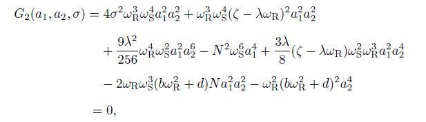 (46)
(46) where σ is the bifurcation parameter,λ and N are the engineering unfolding parameters,and a1 and a2 are the state variables. The transition set is derived by the singularity method as follows[52]:
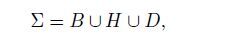 (47)
(47) 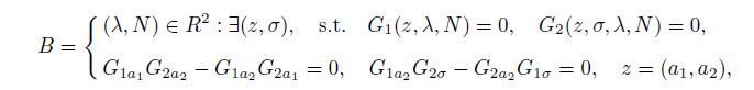 (48)
(48) 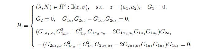 (49)
(49) 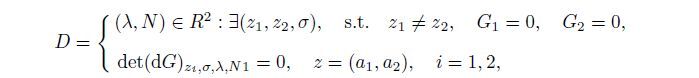 (50)
(50) where B,H,and D represent the bifurcation set,the hysteresis set,and the double limit set,respectively. The partial derivatives of the bifurcation functions G1 and G_2 with respect to σ,a1,and a2 are calculated to obtain the bifurcation sets (see Appendix A for details). Therefore,the transition set of the coupled system can be derived by solving the algebraic equations shown in Eqs.(48)-(50). According to the analysis in Refs.[17],[25],and [43],the other parameters are fixed as follows:

It can be seen from Fig. 4 that the two-parameter space is divided into twelve parts by the transition set,where the red dashed lines denote the bifurcation set,and the blue solid lines present the hysteresis set. Herein the double limit set is D=ø after calculation.

|
| Fig. 4 Transition set,where red dashed lines denote bifurcation sets,andblue lines denote hysteresis sets |
|
|
The transition set can be used to classify different kinds of responses of the system. The responses of the coupled system can display different dynamic characteristics when the van der Pol damping λ and the coupling parameter N are chosen in different parameter subspaces.
The representative frequency-response curves of the system in each region of the two-parameter space shown in Fig. 4 are calculated,and the stability is determined by examining the eigenvalues of the corresponding characteristic equation for Eqs.(38),(40),and (42). The characteristic equation is a triple polynomial as follows:
 (51)
(51) A solution is stable if all of the eigenvalues have negative real parts. It is decided by the Routh-Hurwitz criterion[53] as follows:p1 >0,p3>0,and p1 p2-p3>0.
Figure 5 shows that the amplitudes a1 and a2 of the steady-state solutions are unstable for λ=-0.0639 and N=0.1836 in Region I,and the varying trends of the amplitudes a1 and a2 with respect to the detuning parameter σ are opposite to each other.

|
| Fig. 5 Frequency-response curves in Region I when λ=-0.0639,and N=0.1836 |
|
|
Figure 6 depicts that the trivial solutions of the amplitudes a1 and a2 lose stabilities via a saddle-node bifurcation at SN1,resulting in the occurrence of a two-mode solution. One of the two-mode solution is unstable for both the amplitudes a1 and a2,which has opposite varying trends for the amplitudes a1 and a2 with respect to the detuning parameter σ. The other one of the two-mode solution is unstable until a Hopf bifurcation occurs at H1,resulting in a change of the solutions from unstable to stable. The stable solutions decrease until encounter another saddle-node bifurcation at SN2,leading to a change of the solutions from stable to unstable. Then,the unstable solutions decrease until another Hopf bifurcation occurs at H2,resulting in a change of the solutions from unstable to stable.

|
| Fig. 6 Frequency-response curves in Region II when λ=-0.0372,and N=0.3720 |
|
|
Figure 7 shows that,as the detuning parameter σ increases,the trivial solutions jump to the large unstable solutions via a Hopf bifurcation at σ=0.0183 (see H). Then,the unstable amplitude a1 decreases while a2 increases as σ increases. As σ decreases,the unstable solutions jump to the trivial ones via a saddle-node bifurcation at σ=0.0181 (see SN),leading to a change of the solutions from unstable to stable.

|
| Fig. 7 Frequency-response curves in Region III when λ-0.0043,and N=0.3000 |
|
|
It can be seen from Fig. 8 that as σ increases,the responses increase until encounter a saddle-node bifurcation at SN1,resulting in that the responses jump to the large solutions. The large responses increase until reach the maximum values,then decrease until a saddle-node bifurcation occurs at SN2,leading to that the solutions jump to the small solutions. Then,the responses decrease all the way as σ increases. Similarly,as σ decreases,the amplitudes a1 and a2 have the same varying trends,and encounter two saddle-node bifurcations at SN3 and SN4,

|
| Fig. 8 Frequency-response curves in Region IV when λ=0.0629,and N=0.2178 |
|
|
Figure 9 shows that the amplitudes of the steady-state solutions of the beam and van der Pol oscillator are stable for λ=0.0400 and N=0.0519. Both Fig. 8 and Fig. 9 show that the varying trend of the amplitude a1 with respect to the detuning parameter is the same as that of the amplitude a2.

|
| Fig. 9 Frequency-response curves in Region V when λ=0.0400,and N=0.0519 |
|
|
It can be seen from Fig. 10 that the stable trivial solutions become unstable via a Hopf bifurcation for σ=0.0090.

|
| Fig. 10 Frequency-response curves in Region VI when λ=-0.0013,and N=0.0655 |
|
|
Figures 11-13 show that the solutions in Regions VII-IX are unstable solutions expect the trivial solutions. While the varying trends of the amplitudes a1 and a2 with respect to the detuning parameter σ are opposite in Fig. 11 and the same in Figs. 12 and 13.

|
| Fig. 11 Frequency-response curves in Region VII when λ=-0.0090,and N=0.0315 |
|
|

|
| Fig. 12 Frequency-response curves in Region VIII when λ=-0.0110,and N=-0.0455 |
|
|

|
| Fig. 13 Frequency-response curves in Region IX when λ=-0.0009,and N=-0.0172 |
|
|
It can be seen from Fig. 14 that the trivial solutions jump to the large stable solutions via a Hopf bifurcation at σ= -0.0015 (see H1) as σ increases. Then,the amplitude a1 decreases and the amplitude a2 increases to the trivial solutions as σ increases. While as σ decreases,the amplitude a1 increases and the amplitude a2 decreases until a Hopf bifurcation occurs at σ=-0.0052 (see H2) ,leading to a change of the solutions from unstable to stable. When σ decreases beyond H2,the amplitudes a1 and a2 jump to the trivial solutions.

|
| Fig. 14 Frequency-response curves in Region X when λ=0.0200,and N=-0.1000 |
|
|
It can be seen from Fig. 15 that as σ increases,the amplitude a1 grows while the amplitude a2 decreases all the way until a Hopf bifurcation occurs at σ=0.0045 (see H1),after that,the responses encounter a saddle-node bifurcation at σ=0.0064 (see SN1),resulting in a change of the solutions from unstable to stable. Beyond S_{N1,the amplitude a1 jumps to the small solution,while a2 jumps to the large solution. Then,the amplitude a1 decreases while a2 increases all the way as σ increases. The amplitudes a1 and a2 have symmetrical varying trends as σ decreases.

|
| Fig. 15 Frequency-response curves in Region XI when λ=0.0780,and N=-0.1163 |
|
|
Figure 16 shows that the trivial solutions jump to the stable solutions via a Hopf bifurcation for σ=0.0003. The amplitude a1 jump to the maximum values rapidly. Then,as σ increases,the amplitude a1 decreases while the amplitude a2 increases gradually until to the trivial solutions.

|
| Fig. 16 Frequency-response curves in Region XII when λ=0.0013,and N=-0.0070 |
|
|
The results show that when λ and N have the same signs,i.e.,λ N >0,the varying trends for the structural and van der Pol vibrations are the same with respect to the detuning parameter σ. Specifically,when λ>0 and N>0,the solutions are stable or can encounter the saddle-node bifurcation as σ varies; when λ <0 and N<0,the solutions are unstable as σ varies. When λ and N have opposite signs,i.e.,λ N<0,the varying trends of thetwo coupled motions are reverse to each other,which means the energy transfer between the two modes. The Hopf bifurcation can occur for certain parameter valueswhen λ N<0.
4 Numerical resultsThe response bifurcations of the coupled system including the Hopf and saddle-node bifurcations can occur under certain parameter values as analyzed in the previous section. To verify the validity of the multiple scale method,the characteristics of the dynamic responses for the original systems (17) and (22) are investigated. A representative point (σ=0.0285) after the Hopf bifurcation shown in Fig. 6 is chosen with the unfolding parameters λ=-0.0372 and N=0.3720. The other parameters are fixed as follows:

The time histories,phase portraits,and Lyapunov exponents for the original structural and van der Pol motions with the above parameter values are computed by the Runge-Kutta method (see Figs. 17 and 18). It shows that the largest Lyapunov exponent of the original system with the initial condition values v1(0)=0.05,y(0)=0.00,q1(0)=0.50,and p(0)=0.00 (assuming v1(T)=y(T) and q1(T)=p(T)) tends to zero as time T increases,which means that the quasi-periodic solutions occurs under this parameter conditions. Therefore,the Hopf bifurcation for the modulated solutions indicates the occurrence of the quasi-periodic solutions for the original system,which can result in important physical consequences[54],such as a behavior from transition to chaos.

|
| Fig. 17 Time histories and phase portraits of vibrations for original system at typical point (σ=0.0285) after Hopf bifurcation shown in Fig. 6 with initial conditions v1(0)=0.05,y(0)=0.00,q1(0)=0.504,and p(0)=0.00 when λ=-0.0372,and N=0.3720 |
|
|

|
| Fig. 18 Lyapunov exponents for original system at typical point (σ=0.0285) after Hopf bifurcation shown in Fig. 5 with initial conditions v1(0)=0.05,y(0)=0.00,q1(0)=0.50,and p(0)=0.00 when λ=-0.0372 |
|
|
The saddle-node bifurcation is another bifurcation type analyzed in this paper,which indicates the stability changing of the responses,resulting in the occurrences for the jump phenomenon and multiple solutions. A typical point (σ=0.016) between the two saddle-node bifurcation points when λ=0.0629 and N=0.2178 in Region IV (see Fig. 8) is chosen to obtain two stable solutions by the Runge-Kutta method. The other parameters are fixed as follows:

The two sets of the time histories and phase portraits for the structural and van der Pol motions are obtained with theinitial condition values v1(0)=0.1,y(0)=0.0,q1(0)=2.0,and p(0)=0.0 and v1(0)=0.40,y(0)=0.00,q1(0)=2.65,and p(0)=0.00,respectively,which are shown in Fig. 19.

|
| Fig. 19 Time histories and phase portraits of multiple-solutions when λ=0.0629,N=0.2178,and σ=0.0160,where blue solid lines indicate vibrations with initial condition values v1(0)=0.1,y(0)=0.0,q1(0)=2.0,and p(0)=0.0,and red dotted lines remark vibrations with initial condition values v1(0)=0.40,y(0)=0.00,q1(0)=2.65,and p(0)=0.00 |
|
|
Moreover,the time histories of the two-degree-of-freedom motions can be predicted by Eqs.(24),(29),and (38)-(41) analytically. The comparisons of the time histories obtained by the analytical and numerical methods for the two different solutions shown in Fig. 19 are carried out with the same system parameter values as follows:

Figures 20 and 21 show that the analytical results for the time histories agree with the numerical results obtained by the Runge-Kutta method.

|
| Fig. 20 Comparisons of time histories obtained with analytical and numerical methods when λ=0.0629,N=0.2178,and σ=0.0160 with initial conditions v1(0)=0.1,y(0)=0.0, q1(0)=2.0,and p(0)=0.0,where solid lines and circled lines denote analytical and numerical results,respectively |
|
|

|
| Fig. 21 Comparisons of time histories obtained by analytical and numerical methods when λ=0.0629,N=0.2178,and σ=0.0160 with initial conditions v1(0)=0.40, y(0)=0.00,q1(0)=2.65,and p(0)=0.00,where solid lines and circled lines denote analytical and numerical results,respectively |
|
|
The vortex-induced vibrations of a rotating blade are investigated. The blade is modelled as a uniform and straight cantilever beam,and the van der Pol oscillator is used to simulate the time-varying of the vortex. The reaction for the motion of the blade on the fluid is represented by a linear inertial coupling. The multiple scale method is used to analyze the 1:1 internal resonance of the coupled system. The bifurcation equations are derived,and a two-parameter bifurcation diagram for the van der Pol damping λ and the coupling parameter N is obtained with the singularity theory of two state variables. The bifurcation characteristics for the frequency-responses in different bifurcation regions are investigated. The phenomena including the saddle-node and Hopf bifurcations are found to occur under certain parameter regions. The bifurcation analysis shows that when the parameters λ and N have the same signs,i.e.,λ N>0,the varying trends of the structural and van der Pol motions are similar to each other. Specifically,when both λ and N are positive,i.e.,λ>0 and N>0,two kinds of dynamic characteristics for the responses can occur,i.e.,(i) the responses are totally stable as σ varies,e.g.,the responses in Region V; (ii) the solutions can encounter the saddle-node bifurcation at a certain value for the detuning parameter σ,e.g.,the responses in Region IV. When both λ and N are negative,i.e.,λ <0 and N<0,the solutions are unstable as σ varies,e.g.,the responses in Region VIII. When λ and N have opposite signs,i.e.,λ N<0,the varying trends of the two motions are opposite to each other,which means the energy transfer between the two modes. The Hopf bifurcation can be encountered for certain parameter values when λ and N have opposite signs. The time histories,phase portraits,and Lyapunov exponents are calculted with the Runge-Kutta method for the original system at a point after the Hopf bifurcation in Region III. The results reveal that the occurrence of the Hopf bifurcation for the modulation equations indicates the quasi-periodic motion for the original system. Additionally,the coexisting multiple solutions generated for the saddle-node bifurcation in the parametric Region IV are illustrated,whilst their corresponding numerical and analytical time histories are compared subsequently,both of which are in good agreement with each other. These results indicate the validity of the analytical solutions obtained by the multiple scale method.
Acknowledge The first author thanks for the hospitality of the University of Aberdeen.| [1] | Williamson, C., H. K. and Roshko, & A Vortex formation in the wake of an oscillating cylinder. Journal of Fluids and Structures, 2, 355-381 (1988) |
| [2] | L, ai, J., C. S. and Platzer, & M., F Jet characteristics of a plunging airfoil. AIAA Journal, 37, 1529-1537 (1999) |
| [3] | Sh, yy, W, ., Be, rg, M, ., and, Ljungqvist, & D Flapping and flexible wings for biological and micro air vehicles. Progress in Aerospace Sciences, 35, 455-505 (1999) |
| [4] | Gostelow, J., P., Platzer, M., F., and, Carscallen, & W., E On vortex formation in the wake flows of transonic turbine blades and oscillating airfoils. Journal of Turbomachinery, 128, 528-535 (2006) |
| [5] | Lawaczeck, O., and Heinemann, & H., J Von Karman vortex streets in the wakes of subsonic and transonic cascades. Unsteady Phenomena in Turbomachinery, 177(28), 1-13 (1975) |
| [6] | Sieverding, C., H. and Heinemann, & H The influence of boundary layer state on vortex shedding from flat plates and turbine cascades. Journal of Turbomachinery, 112, 181-187 (1990) |
| [7] | Beauseroy, P., and Lengelle, & R Nonintrusive turbomachine blade vibration measurement system. Mechanical Systems and Signal Processing, 21, 1717-1738 (2007) |
| [8] | Rodriguez, C., G., Egusquiza, E, ., and, Santos, & I., F Frequencies in the vibration induced by the rotor stator interaction in a centrifugal pump turbine. Journal of Fluids Engineering-Transactions of the ASME, 129, 1428-1435 (2007) |
| [9] | Violette, R, ., de, Langre, E, ., and, Szydlowsky, & J Computation of vortex-induced vibrations of long structures using a wake oscillator model:comparison with DNS and experiments. Computers & Structures, 85, 1134-1141 (2007) |
| [10] | Skaugset, K., B. and Larsen, & C., M Direct numerical simulation and experimental investigation on suppression of vortex induced vibrations of circular cylinders by radial water jets. Flow Turbulence and Combustion, 71, 35-59 (2003) |
| [11] | Guilmineau, E., and Queutey, & P Numerical simulation of vortex-induced vibration of a circular cylinder with low mass-damping in a turbulent flow. Journal of Fluids and Structures, 19, 449-466 (2004) |
| [12] | R, ao, J., S. and Saldanha, & A Turbomachine blade damping. Journal of Sound and Vibration, 262, 731-738 (2003) |
| [13] | Dimitriadis, G, ., Carrington, I., B., Wright, J., R., and, Copper, & J., E Blade-tip timming measurement of synchronous vibrations of rotating bladed assemblies. Mechanical Systems and Signal Processing, 16, 599-622 (2002) |
| [14] | Kumar, S, ., R, oy, N, ., and, Ganguli, & R Monitoring low cycle fatigue damage in turbine blade using vibration characteristics. Mechanical Systems and Signal Processing, 21, 480-501 (2007) |
| [15] | Barron, M., A. and Sen, & M Synchronization of coupled self-excited elastic beams. Journal of Sound and Vibration, 324, 209-220 (2009) |
| [16] | Barron, & M., A Vibration analysis of a self excited elastic beam. Journal of Applied Research and Technology, 8, 227-239 (2010) |
| [17] | C, ao, D., Q., Go, ng, X., C., W, ei, D, ., C, hu, S., M., and, Wang, & L., G Nonlinear vibration characteristics of a flexible blade with friction damping due to tip-rub. Shock & Vibration, 18, 105-114 (2011) |
| [18] | C, hu, S., M., C, ao, D., Q., S, un, S., P., P, an, J., Z., and, Wang, & L., G Impact vibration characteristics of a shrouded blade with asymmetric gaps under wake flow excitations. Nonlinear Dynamics, 72, 539-554 (2013) |
| [19] | Bishop, R., E. D. and Hassan, & A., Y The lift and drag forces on a circled cylinder in a flowing fluid. Proceedings of the Royal Society A:Mathematical, Physical and Engineering Science, 277, 32-50 (1964) |
| [20] | Hemon, & P An improvement of the time delayed quasi-steady model for the oscillations of circular cylinders in cross-flow. Journal of Fluids and Structures, 13, 291-307 (1999) |
| [21] | Gabbai, R., and Benaroya, & H An overview of modelling and experiments of vortex-induced vibration of circular cylinders. Journal of Sound and Vibration, 282, 575-616 (2005) |
| [22] | L, ee, Y, ., Vakakis, A, ., Bergman, L, ., and, McFarland, & M Suppression of limit cycle oscillations in the van der Pol oscillator by means of passive nonlinear energy sinks. Structural Control & Health Monitoring, 13, 41-75 (2006) |
| [23] | Hartlen, R., and Currie, & I Lift-oscillator model of vortex induced vibration. Journal of Engineering Mechanics-ASCE, 96, 577-591 (1970) |
| [24] | Sk, op, R., and Griffin, & O A model for the vortex-excited resonant response of bluff cylinders. Journal of Sound and Vibration, 27, 225-233 (1973) |
| [25] | Facchinetti, M., L., de, Langre, E, ., and, Biolley, & F Coupling of structure and wake oscillators in vortex-induced vibrations. Journal of Fluids and Structures, 19, 123-140 (2004) |
| [26] | |
| [27] | Wa, ng, D, ., Ch, en, Y., S., Wiercigroch, M, ., and, Cao, & Q., J A three-degree-of-freedom model for vortex-induced vibrations of turbine blades. Meccanica (2016) |
| [28] | Wa, ng, D, ., Ch, en, Y., S., H, ao, Z., F., and, Cao, & Q., J Bifurcation analysis for vibrations of a turbine blade excited by air flows. Science China Technological Sciences, 59, 1-15 (2016) |
| [29] | Williamson, C., H. K. and Govardhan, & R A brief review of recent results in vortex-induced vibrations. Journal of Wind Engineering and Industrial Aerodynamics, 96, 713-735 (2008) |
| [30] | Kadlec, R., A. and Davis, & S., S Visualization of quasiperiodic flows. AIAA Journal, 17, 1164-1169 (1996) |
| [31] | Ohashi, H., and Ishikawa, & N Visualization study of a flow near the trailing edge of an oscillating airfoil. Bulletin of JSME, 15, 840-845 (1972) |
| [32] | Koochesfahani, & M., M Vortical patterns in the wake of an oscillating airfoil. AIAA Journal, 27, 1200-1205 (1989) |
| [33] | Young, J., and Lai, & J., C. S Oscillation frequency and amplitude effects on the wake of a plunging airfoil. AIAA Journal, 42, 2042-2052 (2004) |
| [34] | Pesheck, E, ., Pierre, C, ., and, Shaw, & S., W Modal reduction of a nonlinear rotating beam through normal modes. Journal of Vibration and Acoustics, Transactions of the ASME, 124, 229-236 (2002) |
| [35] | Ozgür, T., and Gökhan, & B On nonlinear vibrations of a rotating beam. Journal of Sound and Vibration, 322, 314-335 (2009) |
| [36] | X, u, Z, ., L, i, X, ., Pa, rk, J., P., and, Ryu, & S., J Effecr of Coriolis acceleration on dynamic characteristics of high speed spinning steam turbine blades. Journal of Xi'an Jiaotong University, 37, 894-897 (2003) |
| [37] | |
| [38] | Sk, op, R., A. and Balasubramanian, & S A new twist on an old model for vortex-excited vibration. Journal of Fluids and Structures, 11, 395-412 (1997) |
| [39] | Srinil, N, ., Wiercigroch, M, ., and, O'Brien, & P Reduced-order modelling of vortex-induced vibration of catenary riser. Ocean Engineering, 36, 1404-1414 (2009) |
| [40] | X, ue, H, ., Ta, ng, W, ., and, Zhang, & S Simplified model for evaluation of VIV-induced fatigue damage of deepwater marine risers. Journal of Shanghai Jiaotong University, 14, 435-442 (2009) |
| [41] | Facchinetti, M., L., de, Langre, E, ., and, Biolley, & F Vortex-induced travelling waves along a cable. European Journal of Mechanics, Series B, Fluids, 23, 199-208 (2004) |
| [42] | Facchinetti, M., L., de, Langre, E, ., and, Biolley, & F Vortex shedding modelling using diffusive van der Pol oscillators. Comptes Rendus Mecanique, 330, 451-456 (2002) |
| [43] | |
| [44] | H, ao, Z., and Cao, & Q The isolation characteristics of an archetypal dynamical model with stablequasi-zero-stiffness. Journal of Sound and Vibration, 340, 61-79 (2015) |
| [45] | H, ao, Z, ., C, ao, Q, ., and, Wiercigroch, & M Two-sided damping constraint control strategy for highperformance vibration isolation and end-stop impact protection. Nonlinear Dynamics (2016) |
| [46] | Nayfeh, A., H. .Mook, & D., T Nonlinear Oscillations. Wiley-Interscience, New York, 331-338 (1979) |
| [47] | Wa, ng, Y., and Li, & F Nonlinear primary resonance of nano beam with axial initial load by nonlocal continuum theory. International Journal of Non-Linear Mechanics, 61, 74-79 (2014) |
| [48] | B, i, Q., S. and Chen, & Y., S Bifurcation analysis of a double pendulum with internal resonance. Applied Mathematics and Mechanics (English Edition), 21(3), 255-264 (2000) |
| [49] | Chen, Y. S. and Leung, A. Y. T. Bifurcation and Chaos in Engineering, Springer-Verlag, London ,1998 |
| [50] | Golubitsky, M. and Schaeffer, D. G. Singularities and Groups in Bifurcation Theory, SpringerVerlag, New York ,1984 |
| [51] | Wa, ng, X., D., Ch, en, Y., S., and, Hou, & L Nonlinear dynamic singularity analysis of two interconnected synchronous generator system with 1:3 internal resonance and parametric principal resonance. Applied Mathematics and Mechanics (English Edition), 36(8), 985-1004 (2015) |
| [52] | Q, in, Z., H., Ch, en, Y., S., and, Li, & J Singularity analysis of a two-dimensional elastic cable with 1:1 internal resonance. Applied Mathematics and Mechanics (English Edition), 31(2), 143-150 (2010) |
| [53] | Schmidt, G. and Tondl, A. Nonlinear Vibration, Cambrige University Press, Cambrige ,1986 |
| [54] | Monteil, M, ., Touzé, C, ., Thomas, O, ., and, Benacchio, & S Nonlinear forced vibrations of thin structures with tuned eigenfrequencies:the cases of 1:2:4 and 1:2:2 internal resonances. Nonlinear Dynamics, 75, 175-200 (2014) |