 2016, Vol. 37
Shanghai University
Article Information
- Jianzhong LIN, Xiaojun PAN, Zhaoqin YIN, Xiaoke KU
- Solution of general dynamic equation for nanoparticles in turbulent flow considering fluctuating coagulation
- Applied Mathematics and Mechanics (English Edition), 2016, 37(10): 1275-1288.
- http://dx.doi.org/10.1007/s10483-016-2131-9
Article History
- Received Jan. 6, 2016
- Revised Mar. 30, 2016


2. Institute of Fluid Mechanics, China Jiliang University, Hangzhou 310018, China
Nanoparticulate flows occur in a wide range of natural phenomena and engineering applications such as heat transfer enhancement, drag reduction, drug delivery system, and detection of proteins. There are two approaches to examine the modeling of nanoparticle evolution, namely, Eulerian and Lagrangian. In general, computational demand of an Eulerian method appears to be much less than that with a Lagrangian method. In the Eulerian framework, the starting point lies within the following general dynamic equation (GDE) which can include nucleation, coagulation, condensation, breakage, and so on.
In many cases of practical interests, the fluid in which the nanoparticles are suspended is in turbulent motion. In this case, the effect of turbulence on the particle convection, diffusion, nucleation, and coagulation should be accounted for. Some investigations have been performed to study the nanoparticle evolution in turbulent flow based on the GDE. Schwarzer et al.[1] investigated the impact of various process steps on the resulting particle size distribution as representative property using barium sulfate as exemplary material. Process simulations were carried out by solving the population balance equation coupled to a model describing the micromixing kinetics. Shear-induced agglomeration was found to be controllable through the residence time in turbulent regions and the intensity of turbulence, necessary for intense mixing but undesired due to agglomeration. Di Veroli and Rigopoulos[2] presented a methodology for modeling turbulent precipitation using the concept of the transported probability density function in conjunction with a discretized population balance equation, simulated via a Lagrangian stochastic method. Such an approach resolves the closure problem of turbulent precipitation for arbitrarily complex precipitation kinetics, while retrieving the full particle size distribution. Eitzlmayr et al.[3] developed a model for the prediction of polyacrylic acid/protamine nanoparticle precipitation to constitute the first numerical approach for modeling the precipitation of organic nanoparticles. Population balance equations, accounting for nucleation, growth, and aggregation, were used and coupled with the engulfment model for mixing. It was found that the formation of the electrostatic surface charge cannot be described instantaneously. Loeffler et al.[4] performed large eddy simulations of titanium dioxide nanoparticles in three-dimensional turbulent reacting planar jets. The spatio-temporal evolution of the particle field was obtained by utilizing a nodal representation of the GDE. Gradient-diffusion and Smagorinsky-type subgrid-scale closures were used to account for the unresolved stresses, fluid-scalar fluxes, and fluid-particle fluxes. The results suggested that as the precursor concentration increases, neglect of the unresolved particle-particle interactions may act to increasing the nanoparticle growth-rate. Garrick[5] studied quantitatively and qualitatively the effects of fluid turbulence on the coagulation of aerosols. Direct numerical simulation data were used to isolate the effect of the small or subgrid-scale particle-particle interactions on nanoparticle coagulation in three-dimensional flows. The results showed that small-scale interactions act to both increasing and decreasing particle growth. The contribution of the small-scale interactions primarily acts to reducing particle growth in regions characterized by fluid rotation. Akroyd et al.[6] investigated the first part of a two-stage methodology for the detailed fully coupled modelling of nanoparticle formation in turbulent reacting flows using a projected field method to approximate the joint composition probability density function transport equation that describes the evolution of the nanoparticles. The results showed that inception occurs in a mixing zone near the reactor inlets. Most of the nanoparticle mass is due to surface growth downstream of the mixing zone with a narrower size distribution occurring in the regions of higher surface growth. Soos et al.[7] studied onset of gel formation upon mixing between colloidal dispersions and coagulant solutions in turbulent jets using population balance equation. To describe the interaction between turbulence fluctuations and particle aggregation, a micromixing model based on presumed probability density function was built. The results were presented in the parameter space of the primary particle diameter and the solid volume fraction where strong interplay between mixing and aggregation mechanisms controls the gelation phenomena and consequently also the fluid dynamics. Guichard et al.[8] studied the modeling of the dynamics of nano-aerosols under Brownian motion and turbulence effects based a population balance equation. The results revealed the necessity to take into consideration the Brownian and turbulence effects together in the coagulation kernel and also highlighted the need to introduce the fractal dimension of aggregates.
The GDE for turbulent flow is derived by making the Reynolds assumption that the fluid velocity and size distribution functions can be written as the sum of mean and fluctuating components. When the particle coagulation is considered, the fluctuating coagulation term which is the contribution to coagulation resulting from the fluctuating concentrations will appear after averaging the equation. In the previous studies, the fluctuating coagulation term, consisting of correlation between two fluctuating particle size distribution functions, is neglected. In this study, therefore, the new averaged GDE for nanoparticles in turbulent flow is derived by considering the combined effect of convection, Brownian diffusion, turbulent diffusion, turbulent coagulation, and fluctuating coagulation. As an application, the new GDE is transferred to moment equations which are solved with the Taylor-series expansion moment method in a turbulent pipe flow. As a new GDE for turbulent flow, it must be verified and validated. The experiments are performed, and the numerical results are compared with the experimental ones.
2 GDE for nanoparticles 2.1 Averaged GDE for nanoparticlesThe evolution of nanoparticles is related to the convection, diffusion, coagulation, and so on. Coagulation is a process, whereby particles collide with one another and adhere to form large particles, resulting in the nanoparticle size increased and particle number density decreased. The evolution of nanoparticles in the flow is governed by the GDE. The instantaneous GDE for nanoparticles under the combined effect of convection, diffusion, and coagulation is

On the right-hand side, the first and second terms are the birth and death of particles due to coagulation, respectively, $n(v$, $t)$ is the particle size distribution function, μ is the fluid velocity vector, $\beta $($v$, $v_{1})$ is the coagulation kernel for two particles of volume $v$ and $v_{1}$, and $D$ is the particle diffusion coefficient which can be given as[9]

where $k_{\rm B}$ is the Boltzmann constant, $T$ is the temperature, $Kn$ is the Knudsen number $(Kn = \lambda /{r_{\rm{p}}}$, in which $\lambda $ is the gas molecular mean free path, and $r_{\rm p}$ is the particle radius), $\mu$ is the dynamic viscosity of fluid, and $ d_{\rm p}$ is the particle diameter.
The GDE for nanoparticles in the turbulent flow is derived by making the Reynolds assumption that the fluid velocity and particle size distribution functions can be written as the sum of mean and fluctuating components,

Substituting Eq. (3) into Eq. (1) and averaging with respect to time, we have

As a result of time averaging, several new terms appear in Eq. (4) . The last term on the left-hand side is a form that represents the change in $\bar {n}$ resulting from turbulent diffusion. The separate components of the vector flux $n'$μ' are usually assumed to be[9]

in which the eddy diffusivity $\nu$$_{\rm t}$ can be obtained by solving the equations of turbulent flow. The third and fourth terms on the right-hand side of Eq. (4) , called the fluctuating coagulation term, are the contribution to coagulation resulting from the fluctuating concentrations and are neglected in the previous studies[9]. Here, we make an assumption that the correlation of fluctuating concentration is related to the mean concentration, the mean flow kinetic energy, and the turbulent kinetic energy as follows:

which $k$ is the turbulent kinetic energy. When the flow is laminar, the turbulent kinetic energy $k$ is zero, and the fluctuating coagulation terms disappear.
Thus, substituting Eqs. (5) and (6) into Eq. (4) , we obtain

Equation (7) is the averaged GDE for nanoparticles in the turbulent flow under the effect of convection, Brownian diffusion, turbulent diffusion, and particle coagulation.
2.2 Particle coagulation kernelThe particle coagulation kernel $\beta $($v$, $v_{1})$ in Eq. (7) should be defined in advance. The particle coagulation is induced by Brownian motion and laminar and turbulent shear. Turbulent coagulation generally becomes important for particles lager than a few microns but may be significant for submicron particles in turbulent flows[9]. Ounis and Ahmadi[10] pointed out that particle diffusion is generally dominated by turbulence dispersion, and the Brownian diffusion has no significant effect on the particle response statistics. Therefore, we consider the turbulent shear-induced coagulation[11],

where $\varepsilon $ is the turbulent dissipation rate, and $\nu$ is the kinematic viscosity of fluid.
3 Moment equation for nanoparticles and moment method 3.1 Moment equation for nanoparticlesThe GDE has only several known analytical solutions due to its own complexity. Therefore, numerical method has to be used to obtain approximate solutions. However, the direct numerical simulations become impractical due to the requirement of large computational cost. For breaking the limit in computational cost, three methods, i.e., the moment method, the sectional method, and the stochastic particle method, are usually used. Among the three methods, the moment method has been widely used because of its relative simplicity of implementation and low computational cost. The moment method is based on the moment equation, and the general moment of the particle size distribution function is defined by

where the index number $j$ represents the order of the moment. Many of the moments appear in expressions for the particle physical or optical properties, or transport rates. The zero moment, $m_{0}$, corresponds to the particle number concentration, which decreases as the particle grows. The first moment, $m_{1}$, is proportional to total particle mass. The second moment, $m_{2}$, increases as the mean particle size and polydispersity increase.
Using the expression (9) , we can transform Eq. (7) into an ordinary differential equation with respect to the moment $m_{j}$. The moment transformation involves multiplying Eq. (7) by $v^{j}$ and then integrating over the entire size distribution,
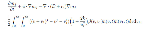 (10)
(10) Equation (10) is the moment equation for nanoparticles in the turbulent flow.
3.2 Taylor-series expansion moment methodGreat efforts have been made to achieve the closure of moment equation using different moment methods, for example, Pratsinis's log-normal moment method, approximating the integral moment by an $n$-point Gaussian quadrature, assuming the $p$th-order polynomial form for the moments, achieving closure with interpolative method and Taylor-series expansion method of moment (TEMOM). The TEMOM achieves the closure of moment equation based on the Taylor-series expansion technique[12] and has been effectively used[13-17].
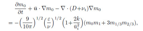
Substituting Eq. (8) into Eq. (10) with $j=0$, 1, 2, and using the TEMOM, we have
 (11a)
(11a) 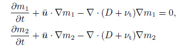 (11b)
(11b) 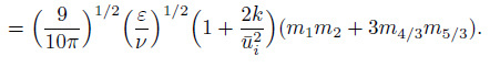 (11c)
(11c) Equation (11) consists of integral and fractional order moments. In order to close Eq. (11) , the fractional order moments should be disposed by continuously using the Taylor-series expansion technique with respect to the fractional $j$th moment. $v^{j}$ in Eq. (9) can be expanded with Taylor-series about the point $v=w$, which is consistent with the expansion point $w$ in ($v$+$v_{1})^{1/2}$,
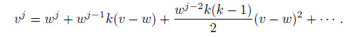 (12a)
(12a) Truncating Eq. (12a) and remaining the first three terms of Taylor-series, we have
 (12b)
(12b) Substituting Eq. (12a) into Eq. (9) yields[12]
 (12c)
(12c) in which $v=m_{1}$/$m_{2}$ is the particle volume. The final form of moment equations can be obtained by substituting Eq. (12c) into Eq. (11) ,
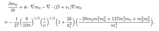 (13a)
(13a) 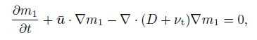 (13b)
(13b) 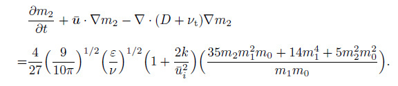 (13c)
(13c) We apply the model and equations mentioned above to a turbulent pipe flow to prove the availability of the model and equations, and the experiments are performed to validate the numerical results.
4.1 Flow fieldThe nanoparticulate pipe flow and the coordinate system are shown in Fig. 1. The flow is considered as an incompressible and fully developed turbulent. The continuity equation and the Reynolds averaged Navier-Stokes equation are
 (14)
(14)  (15)
(15) where $\bar{u}_i$ and $\bar{p}$ are the mean fluid velocity and pressure, respectively, $\rho $ is the fluid density, $\nu $ is the kinematic viscosity of fluid, and $-\rho \overline {{u}'_i {u}'_j } $ is the Reynolds stress,
 (16)
(16) in which the eddy viscosity $\mu_{\rm T} =0.09\rho k^2/\varepsilon $, $k$ is the turbulent kinetic energy, and $\varepsilon $ is the turbulent dissipation rate. The corresponding equations are
 (17)
(17) 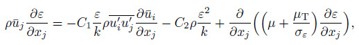 (18)
(18) where $\mu $ is the dynamic viscosity of fluid, $C_{1}$=1.44, $C_{2}$=1.92, $\sigma $$_{k} =$1.0, and $\sigma $$_{\varepsilon } =$1.3.

|
| Fig. 1 Pipe flow and coordinate system |
|
|
In the computation, the grid system consists of 60($r)\times 50(\theta )\times $100($z)$=300~000 grid points in a cylindrical coordinate system. For guaranteeing a higher mesh resolution in the near-wall region, the size of the cells is set to increase geometrically by a factor of 1.1 in the radial direction from the wall to the centerline. The wall effect is considered through a wall function suggested by Kader[18]. The extensive tests and refinements of the independence and suitability of the grid size for the convergence results are performed, i.e., the relative difference between the numerical results of $m_{j}$ for different grid resolutions is less than 10$^{-3}$. Equation (13) is solved using an explicit finite difference scheme which is first order accurate in time and second order accurate in space. Some parameters are as follows: $\rho =1.205$ kg/m$^{3}$, $\nu=1.5\times $10$^{-5}$ m$^{2}$/s, $T=293$ K, and $k=1.38\times $10$^{-23}$~J/K.
4.3 Experiment set-upThe experiments are performed to validate the new GDE and method. The experimental test system is depicted schematically in Fig. 2. The particles are generated from the burning of incense and injected into the pressure vessel in which the resulting particles are mixed with clean dilution air. The test section consists of a plexiglass pipe with the inner radius $a=0.6$ cm and the length $l=210$ cm. The experiments are carried out at the temperature of $T=293$ K.

|
| Fig. 2 Schematic of experiment set-up |
|
|
The fast mobility particle sizer (FMPS), based on an electrical mobility detection technique, is used to measure the particle number and size distribution at the inlet and the outlet of the test section. The FMPS system consists of three components: (i) a bipolar radioactive charger for charging the particles, (ii) a differential mobility analyzer for classifying particles by electrical mobility, and (iii) multiple, low-noise electrometers for particle detection. The FMPS system, with a sampling frequency of 1 Hz and duration of 1 min for each measurement, is capable of detecting particles with the diameter ranging from 5.6 nm to 560 nm using 32 channels (16 channels per decade of size). To ensure accurate measurement, each experiment has been repeated at least three times with essentially the same results.
5 Results and discussion 5.1 Particle size distributionParticle coagulation makes particles change their sizes and results in the difference in particle size between the outlet and the inlet. The particle diameter $d_{\rm p}$ can be determined by the zeroth and first moments,
 (19)
(19) Particle size distributions are shown in Fig. 3, in which both the numerical and experimental results are given. In the figure, the curve shapes remain unchanged, and the peak appears around $d_{\rm p}$=180 nm. The numerical results considering the fluctuating coagulation are closer to the experimental results without considering the fluctuating coagulation. Comparing the particle size distribution at the outlet and the inlet, it can be found that the number of small particles decreases drastically at the outlet.

|
| Fig. 3 Particles size distribution (Re=4~200 and $l$/$a$=350) fig 4 Particles size distribution (Re= 5 300 and $l$/$a$=350) |
|
|
Figure 4 shows the particle size distributions at a higher Reynolds number than that in Fig. 3. It can be seen that the peak also appears around $d_{\rm p}$=180 nm, and the difference in the numerical results with and without considering the fluctuating coagulation is more obvious than that in Fig. 3. The flow fluctuation degree is directly proportional to the turbulent degree as well as the Reynolds number. Therefore, it is concluded that the fluctuating coagulation term in the particle GDE should be included in the flow with higher Reynolds numbers.
2.1.2 Particle size distribution along radial direction at outletIf we give an initially particle field with the same diameter at the inlet, the particle size distribution will change when these particles flow through the pipe. The particle size distributions along the radial direction for different Schmidt numbers are shown in Fig. 5, in which $d_{\rm p}$/$d_{\rm p0}$ means the ratio of particle diameter at the outlet to that at the inlet, and $R$ is the radius of pipe. Here, the Schmidt number is defined as
 (20)
(20) where $\nu $ is the kinematic viscosity of fluid, and $D$ is the particle diffusion coefficient as shown in Eq. (2) .

|
| Fig. 5 Particle size distributions along radial direction for different Sc (Re=5 300 and $l/a$=350) |
|
|
From Fig. 5, we can see that the particle size increases from the inlet to the outlet because of coagulation. At the outlet, along the radial direction, the particle size increases from the pipe center to the near-wall region. Particle coagulation is dependent on the mean velocity gradient and the turbulent dissipation rate $\varepsilon $. As shown in Eq. (8) , the turbulent coagulation rate is directly proportional to $\varepsilon $, and the mean velocity gradient and $\varepsilon $ are the largest in the near-wall region, as shown in Fig. 6. Hence, particle coagulation occurs more frequently. Conversely, the shear rate of the mean velocity and $\varepsilon $ are the smallest in the region near the pipe center where the particle coagulation seldom occurs.

|
| Fig. 6 Distributions of velocity and turbulent dissipation rate along radial direction (Re=5 300 and $l/a$=350) |
|
|
Comparing the particle size distributions at the outlet with those at the inlet, we can see that the larger the Schmidt number is, the smaller the value of $d_{\rm p}$/$d_{\rm p0}$ is. The larger particles have a larger Schmidt number as shown in Eq. (20) because larger particles have a smaller diffusion coefficient. Larger particle number concentration is lower when the total particle mass remains the same. Therefore, the larger particles have less chance to coagulate with other particles, and hence have a smaller value of $d_{\rm p}$/$d_{\rm p0}$. When the fluctuating coagulation is considered, the particle sizes are larger at the outlet than those without considering the fluctuating coagulation, because the turbulent fluctuation also contributes to the particle coagulation.
Figure 7 shows the particle size distribution along the radial direction for different Reynolds numbers. The higher the Reynolds number is, the larger the value of $d_{\rm p}$/$d_{\rm p0}$ is. We can also see that the difference in the numerical results with and without considering the fluctuating coagulation is more obvious when the Reynolds number is higher.

|
| Fig. 7 Particle size distributions along radial direction for different Re (Sc=23~428 and $l/a$=350) |
|
|
Table 1 gives the experimental and numerical results of particle mean diameter $d_{\rm a}$ and geometric standard deviation $\sigma_{\rm g}$ at two Reynolds numbers. In the experiment, the particles with the mean diameters of 157.2 nm and 117.9 nm and the geometric standard deviation of 2.14 and 2.02 are injected into the pipe. At the outlet, the particle mean diameter increases because of coagulation. The numerical results of the particle mean diameter and the geometric standard deviation are closer to the experimental ones considering fluctuating coagulation than those without considering fluctuating coagulation. Such phenomenon is more obvious for higher Reynolds number flow. The ratios of particle mean diameter at the outlet to that at the inlet are 1.094 and 1.111, respectively, for $Re=4~200$ and 5~300, which demonstrates that particle coagulation occurs more frequently for higher Reynolds number flows.

The distribution of the zero moment, $m_{0}$, along the radial direction for different Schmidt numbers is shown in Fig. 8, where $m_{0}$/$m_{00}$ means the ratio of particle number concentration at the outlet to that at the inlet. At the outlet, the distribution of $m_{0}$ is non-uniform along the radial direction, and the values of $m_{0 }$ are larger and smaller than those at the inlet in the region of $0\le r/R\le$ 0.52 and $0.52<r/R\le 1$, respectively. The distribution of particle number concentration is dependent on the diffusion and coagulation induced by the Brownian motion and flow shear-induced force. The Brownian motion causes the particles diffuse from a region of higher concentration to that of lower concentration. Therefore, the diffusion of particles with the initial uniform distribution of number concentration is mainly attributed to the flow shear-induced force which is proportional to the mean velocity gradient and turbulent dissipation rate. There exists larger mean velocity gradient and turbulent dissipation rate in the region of $0.52<r/R\le 1$, as shown in Fig. 6. Therefore, particles are diffused from this region to the region of $0\le r/R\le0.52$. As far as coagulation is concerned, the turbulent dissipation rate $\varepsilon $ is larger in the region of $0.52<r/R\le 1$. Hence, particle coagulation occurs more frequently because the coagulation rate is directly proportional to $\varepsilon $. Both factors result in the decrease and increase of particle number concentration in the region of $0.52<r/R\le 1$ and $0\le r/R\le 0.52$, respectively. Lam et al.[19] found that, for micro-sized particles, the particle number concentration was the lowest at the wall, rapidly increased to the maximum at $r/R=0.85$, but decreased slightly towards the pipe center. It can be concluded that the distribution of nanoparticle number concentration is different from that of the microparticle number concentration.

|
| Fig. 8 Distribution of zeroth-order moment along radial direction for different Sc (Re=5 300 and $l/a$=350) |
|
|
As shown in Fig. 8, the larger the Schmidt number is, the larger the difference in particle number concentration between the near-wall region and the near-center region is. This is attributed that the turbulent dissipation rate $\varepsilon $ is related to the Kolmogorov scale in the turbulent flow, and such a scale is closer to the size of particle with larger Schmidt numbers. Therefore, the effect of $\varepsilon $ on the particle diffusion and coagulation is more significant.
The difference in the particle number concentration between the near-wall and near-center regions is larger considering the fluctuating coagulation than that without considering the fluctuating coagulation, because the flow fluctuating plays an additional role in the particle coagulation. The comparison of results for different Reynolds numbers is shown in Fig. 9, from which, we can see the relationship of the Reynolds number and the distribution of particle number concentration. The higher the Reynolds number is, the larger the difference in the particle number concentration between the near-wall and near-center regions is. The reason is that higher Reynolds number corresponds to a larger turbulent dissipation rate $\varepsilon $, and hence stronger diffusion and more frequent particle coagulation.

|
| Fig. 9 Distribution of zeroth-order moment along radial direction for different Re (Sc=23 428 and $l/a$=350) |
|
|
The second moment, $m_{2}$, is directly proportional to the particle polydispersity. Figures 10 and 11 show the distributions of $m_{2}$ along the radial direction for different Schmidt numbers and Reynolds numbers, respectively. $m_{2}$/$m_{20 }$ means the ratio of particle polydispersity at the outlet to that at the inlet. Particle coagulation makes initially monodisperse particles change their sizes and become polydisperse. The curves in Figs. 10 and 11 are similar to that of particle size distribution as shown in Fig. 5. Particle polydispersity increases from the near-center region to the near-wall region where particle coagulation occurs more frequently and hence shows a higher polydispersity. The particles with smaller Schmidt number and the flow with higher Reynolds number show a higher polydispersity at the outlet, as shown in Figs. 10 and 11, respectively. The degree of particle polydispersity is higher considering fluctuating coagulation than that without considering fluctuating coagulation.

|
| Fig. 10 Distribution of second-order moment along radial direction for different Sc (Re=5 300 and $l/D_{\rm p}$=350) |
|
|

|
| Fig. 11 Distribution of second-order moment along radial direction for different Re (Sc=23 428 and $l/D_{\rm p}$=350) |
|
|
The new averaged GDE for nanoparticles in the turbulent flow is derived by considering the combined effect of convection, Brownian diffusion, turbulent diffusion, turbulent coagulation, and fluctuating coagulation. The new averaged GDE is transferred to moment equations which are solved with the Taylor-series expansion moment method in a turbulent pipe flow. The experiments are performed, and the numerical results are compared with the experimental ones. The main conclusions are summarized as follows.
(i) The numerical results of the particle size distribution, the particle mean diameter, and the geometric standard deviation at the outlet are closer to the experimental ones considering fluctuating coagulation than those without considering fluctuating coagulation, which is more obvious for higher Reynolds number flows. Therefore, the fluctuating coagulation term in the averaged particle GDE should be included in the turbulent nanoparticulate flow, especially in the higher Reynolds number flow.
(ii) The number of small particles decreases drastically at the outlet. At the outlet, the particle size increases from the pipe center to the near-wall region. The larger the Schmidt number is and the lower the Reynolds number is, the smaller the value of ratio of particle diameter at the outlet to that at the inlet is.
(iii) At the outlet, the particle number concentration increases from the near-wall region to the near-center region, even though the distribution of particle number concentration is assumed to be uniform at the inlet, which is different from the distribution of microparticle number concentration. The larger the Schmidt number is and the higher the Reynolds number is, the larger the difference in particle number concentration between the near-wall region and near-center region is.
(iv) At the outlet, the particle polydispersity increases from the near-center region to the near-wall region, even though the particle is assumed to be monodisperse at the inlet. The particles with smaller Schmidt number and the flow with higher Reynolds number show a higher polydispersity. The degree of particle polydispersity is higher considering fluctuating coagulation than that without considering fluctuating coagulation.
| [1] | Schwarzer, H.C., Schwertfirm, F., Manhart, M., Schmid, H.J., & Peukert, W Predictive simulation of nanoparticle precipitation based on the population balance equation. Chemical Engineering Science, 61(1), 167-181 doi:10.1016/j.ces.2004.11.064 (2006) |
| [2] | Di Veroli, G., & Rigopoulos, S Modeling of turbulent precipitation:a transported population balance-PDF method. AICHE Journal, 56(4), 878-892 (2010) |
| [3] | Eitzlmayr, A., Petschacher, C., Radl, S., Suzzi, D., Zimmer, A., & Khinast, J.G Modeling and simulation of polyacrylic acid/protamine nanoparticle precipitation. Soft Matter, 7(19), 9484-9497 doi:10.1039/c1sm05501a (2011) |
| [4] | Loeffler, J., Das, S., & Garrick, S.C Large eddy simulation of titanium dioxide nanoparticle formation and growth in turbulent jets. Aerosol Science and Technology, 45, 616-628 doi:10.1080/02786826.2010.551147 (2011) |
| [5] | Garrick, S.C Effects of turbulent fluctuations on nanoparticle coagulation in shear flows. Aerosol Science and Technology, 45(10), 1272-1285 doi:10.1080/02786826.2011.589482 (2011) |
| [6] | Akroyd, J., Smith, A.J., Shirley, R., McGlashan, L.R., & Kraft, M A coupled CFD-population balance approach for nanoparticle synthesis in turbulent reacting flows. Chemical Engineering Science, 66(17), 3792-3805 doi:10.1016/j.ces.2011.05.006 (2011) |
| [7] | Soos, M., Marchisio, D.L., & Sefcik, J Assessment of gel formation in colloidal dispersions during mixing in turbulent jets. AIChE Journal, 59(12), 4567-4581 doi:10.1002/aic.14268 (2013) |
| [8] | Guichard, R., Taniere, A., Belut, E., & Rimbert, N Simulation of nanoparticle coagulation under Brownian motion and turbulence in a differential-algebraic framework:developments and applications. International Journal of Multiphase Flow, 64, 73-84 (2014) |
| [9] | Friedlander, S, K. Smoke, Dust and Haze:Fundamentals of Aerosol Behavior, Wiley, New york (2000) |
| [10] | Ounis, H., & Ahmadi, G.A A comparison of Brownian and turbulent diffusion. Aerosol Science and Technology, 13, 47-53 doi:10.1080/02786829008959423 (1990) |
| [11] | Saffman, P.G., & Turner, J.S On the collision of drops in turbulent clouds. Journal of Fluid Mechanics, 1, 16-30 doi:10.1017/S0022112056000020 (1956) |
| [12] | Yu, M.Z., Lin, J.Z., & Chan, T.L A new moment method for solving the coagulation equation for particles in Brownian motion. Aerosol Science and Technology, 42, 705-713 doi:10.1080/02786820802232972 (2008) |
| [13] | Yu, M.Z., & Lin, J.Z Nanoparitcle-laden flows via moment method:a review. International Journal of Multiphase Flow, 36(2), 144-151 doi:10.1016/j.ijmultiphaseflow.2009.08.006 (2010) |
| [14] | Yu, M.Z., & Lin, J.Z Solution of the agglomerate Brownian coagulation using Taylor-expansion moment method. Journal of Colloid and Interface Science, 336(1), 142-149 doi:10.1016/j.jcis.2009.03.030 (2009) |
| [15] | Xie, M.L., & Wang, L.P Asymptotic solution of population balance equation based on TEMOM model. Chemical Engineering Science, 94, 79-83 doi:10.1016/j.ces.2013.02.025 (2013) |
| [16] | Wan, Z.H., You, Z.J., Sun, Z.L., & Yin, W.B Method of Taylor expansion moment incorporating fractal theories for Brownian coagulation of fine particles. International Journal of Nonlinear Sciences and Numerical Simulation, 13(7-8), 459-467 (2012) |
| [17] | Lin, P.F., Wu, D.C., Yu, M.Z., Wang, C., & Zhu, Z.F Large eddy simulation of the particle coagulation in high concentration particle laden planar jet flow. Chinese Journal of Mechanical Engineering, 25(1), 1-10 doi:10.3901/CJME.2012.01.001 (2012) |
| [18] | Kader, B.A Temperature and concentration profiles in fully turbulent boundary layers. International Journal of Heat and Mass Transfer, 24(9), 1541-1544 doi:10.1016/0017-9310(81)90220-9 (1981) |
| [19] | Lam, Y.C., Chen, X., Tan, K.W., Chai, J.C., & Yu, S.C Numerical investigation of particle migration in Poiseuille flow of composite system. Composites Science and Technology, 64, 1001-1010 doi:10.1016/j.compscitech.2003.08.005 (2004) |