 2016, Vol. 37
Shanghai University
Article Information
- Wenxin HUAI, Suwen SONG, Jie HAN, Yuhong ZENG
- Prediction of velocity distribution in straight open-channel flow with partial vegetation by singular perturbation method
- Applied Mathematics and Mechanics (English Edition), 2016, 37(10): 1315-1324.
- http://dx.doi.org/10.1007/s10483-016-2135-9
Article History
- Received Feb. 1, 2016
- Revised May. 4, 2016


Vegetation growing in natural rivers not only contributes to the stabilization of river banks, but also helps in ecological restoration. Vegetation increases flow resistance and results in a more complicated flow structure, which retards water flow. The flow depth and the velocity vary with changes in aquatic vegetation types and their distribution in the river. For open channels with partial vegetation, such as riparian vegetation in simple or compound channels, vegetation has a profound effect on the flow characteristics within both the vegetation and non-vegetation regions.
Numerous experiments have been carried out to study the effect of vegetation on flows. Li and Shen[1] concluded that the flow velocity was affected by the planting density and array mode of the vegetation. Tanino and Nepf[2] investigated the drag force exerted by randomly distributed, rigid, and emergent circular cylinders via laboratory experiments. They presented the general range of the drag force coefficient both in a straight and wandering channel. The relationships between the drag force coefficient and the parameters such as the volume fraction were also presented.
Numerical simulations have been presented to predict the complex turbulent flow features in open channels with partially vegetation[3-7]. Shimizu and Tsujimoto[8] simulated the behavior of turbulent flow in a partially vegetated channel with the $k$-$\varepsilon $ model. Van Prooijen and Knight[9] proposed a new eddy viscosity model incorporating horizontal coherent structures and bottom turbulence to evaluate the transverse momentum exchange. Tang and Knight[10] presented a new boundary condition at the interface between the main channel and adjoined floodplain, and the predicted lateral velocity distribution closely matched field measurements. Rameshwaran and Shiono[11] proposed a quasi-two-dimensional model to calculate the depth-averaged velocity and the bed-shear stress in a prismatic channel with an emergent vegetated floodplain, and introduced the vegetation drag term and porosity to investigate the feasibility of this model.
This paper examined the secondary current between the vegetated and non-vegetated regions. The secondary current is caused by the lateral momentum exchange due to velocity differences between the two regions. Shiono and Knight[12] conducted an experimental investigation in a compound channel with partial vegetation. They concluded that the shear stress due to the secondary flow, $\rho (\overline U \overline V )_\mathrm d $, decreased approximately linearly across the interface between the floodplain and the main channel, and $\rho (\overline U \overline V )_\mathrm d $ changed with $\frac{\partial u}{\partial y}$, where $\rho $ is the density of water, $\overline U $ and $\overline V $ are the temporal mean velocity components corresponding to the $x$- and $y$-directions, respectively, $(\overline U \overline V)_\mathrm d =\frac{1}{H}\int_0^H {\overline U \overline V } \mathrm dz$, and $u $ is the depth-averaged streamwise flow velocity. Ervine et al.[13] suggested an analytical model with consideration of the secondary flow term to estimate velocity and shear stress for straight and meandering overbank flow. In their model, a secondary current intensity coefficient was introduced, and the lateral velocity was assumed to be a fraction of the depth-averaged streamwise velocity. Liu et al.[14] applied this model to predict the velocity and the bed shear stress in compound channels, and the results closely matched the experimental data.
Ikeda et al.[15] adopted the singular perturbation method to predict the velocity distribution. The singular perturbation method is an important mathematical tool used in theoretical research and is effective for the analysis of weakly nonlinear problems. It relies on a dimensionless parameter that is relatively small, and approximate solutions can be obtained through the perturbation method. In Ref. [15], the secondary flow at the interface between the vegetation and non-vegetation zones was not included. In this paper, we consider the transverse momentum exchange to improve the prediction accuracy for lateral distribution of streamwise velocity with the singular perturbation method.
2 Theoretical backgroundConsider a straight open channel wide enough to allow cylinders acting as vegetation to be arranged symmetrically on both sides along the flow. The regions occupied by the cylinders are considered as the vegetation region, while the free-flow region between the two vegetated regions is the non-vegetation region. The diameter of each cylinder is small compared with the full width of the channel. Because of its symmetrical nature, the model is simplified by only considering one half of the channel. The rectangular coordinates are shown in Fig. 1.

|
| Fig. 1 Sketch of open channel with lateral partial vegetation |
|
|
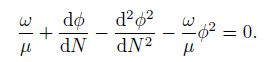
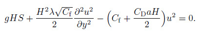
For a uniform steady flow, the depth-averaged momentum equation in the streamwise direction can be simplified as

where $g$ is the gravitational acceleration, $H$ is the local flow depth, $S$ is the longitudinal energy slope, $\varepsilon _y $ is the depth-averaged eddy viscosity, $C_\mathrm f $ is the resistance coefficient, $C_\mathrm D $ means the drag force coefficient, and $a$ is the mean projected area per unit volume.
Analogous with Shiono and Knight's[12] approach in a compound channel, we assume that $\frac{\partial H(\overline U \overline V )_\mathrm d }{\partial y}=E\frac{\partial u}{\partial y}$, where $E$ is a constant. The dimension analysis suggested that $E$ can be replaced by $H \overline {V}'$, where $\overline{V}'$ is the section-averaged lateral velocity. Further, $\overline {V}'$ is replaced by $\overline {V}'=K \overline {U}'$ based on Ervine's assumption, where $\overline {U}'$ is the section-averaged velocity, and $K$ is the secondary current intensity coefficient accounting for the intensity of the secondary cell. We assume that the lateral velocities in the two sections both flow toward the interface, i.e., $\overline {V}'=-| K| \overline {U}'$ in the non-vegetation and $\overline {V}'=| K| \overline {U}'$ in the vegetation. $\varepsilon _y $ can be replaced by $\lambda HU_\ast $, where $\lambda $ is the lateral dimensionless eddy viscosity, and $U_\ast =\sqrt {C_{\mathrm f } u} $ is the friction velocity. Thus, Eq. (1) can be expressed as


In the region laterally far away from the vegetation, Eq. (2) reduces to

Divide Eqs. (2) and (3) by Eq. (2) , respectively,


where

$\omega$ is very small, and then the singular perturbation method can be applied.
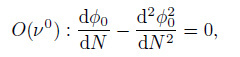
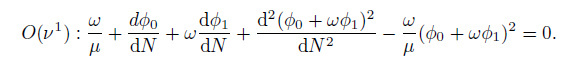
Further, the variable $\phi $ can be expanded with respect to the small perturbation parameters as follows:

where $\phi _0 $ and $\phi _1 $ mean the solutions of $\phi $ in 0th and 1st order, respectively. Substitution of Eq. (7) into Eq. (5) yields


Solving the equations yields
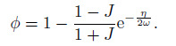
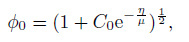 (10)
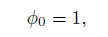
(10) where $\eta =0$, and $\phi =1$. Therefore, $\phi _0 =1$, and $\phi _1 =0$.
For the non-vegetation zone, another independent variable should be introduced to obtain the inner solution near $\eta =0$. The most suitable variable is $\eta =\omega N$. Then, Eq. (5) can be written as
 (11)
(11) Substitution of Eq. (7) into Eq. (11) yields
 (12)
(12)  (13)
(13) The inner solutions are
 (14)
(14) 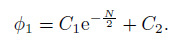 (15)
(15) Matching the inner and outer solutions allows us to solve the momentum equation as
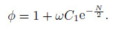 (16)
(16) The solution for the vegetation zone is derived in a similar way
 (17)
(17) The constant $C_{1}$ and $C_{3 }$ can be determined by matching at the boundary $N=0$. The dimensionless velocities $\phi $ and $\mathrm d\phi /\mathrm dN$ are matched at the boundary. Then, the solutions for the region without vegetation are reduced to
 (18)
(18) For the vegetation zone,
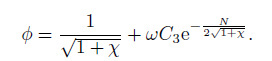
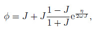 (19)
(19) where $J=1/\sqrt {1+\chi } $.
If the secondary current is ignored, the momentum equation can be written as follows:
 (20)
(20) The numerical solutions for Eq. (20) are
 (21)
(21)  (22)
(22) The data of White and Nepf[16] are selected to verify the predictions (see Table 1). Their experiment was carried out in a 13 m long and 1.2 m wide straight channel with rigid emergent vegetation along one side of the channel. The plants are wooden circular cylinders with a diameter of 6.5 mm, and the width of the vegetation zone is 40 cm. The velocities are measured by laser Doppler velocimetry (LDV).

According to the experimental research of Ervine et al.[13] on the secondary flow in straight channels, the secondary current coefficient $K$ ranged from 2% and 4%. Here, $|K |=3% $ is adopted. The research of Tang and Knight[10] showed that the lateral dimensionless eddy viscosity $\lambda $ varied from 0.067 to 0.7, and here $\lambda =0.25$ is selected by calibration.
The measured and predicted velocities from Eqs. (18) --(19) (with consideration of secondary currents) and from Eqs. (21) --(22) (without consideration of secondary currents) are plotted in Fig. 2.

|
| Fig. 2 Lateral distributions of $u$ |
|
|
Figure 2 clearly shows that the model with consideration of the secondary flow agrees better with the experimental data compared with the model without the secondary flow, especially in the non-vegetation zone adjacent to the interface between the vegetation and non-vegetation zones.
3.2 Reynolds stressThrough Eliana's[17] research, the Reynolds stress can be calculated by the equation
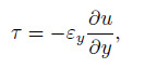 (23)
(23) where $\varepsilon _y =\lambda U_\ast H$. With the predicted velocity from Eqs. (18) --(19) (with consideration of the secondary current term), the Reynolds stress is obtained from Eq. (23) with the same $\lambda = 0.25$. Three cases are chosen for verification (see Fig. 3).
|
|
| Fig. 3 Lateral distributions of Reynolds stress |
|
|
It can be seen from Fig. 3 that the Reynolds stress reaches a peak value at the interface between the vegetation and non-vegetation zones because the turbulence is the strongest here. In the vegetation zone, the Reynolds stress decreases sharply from its maximum to zero, which suggests that the turbulence cannot penetrate deeply into the vegetation zone.
4 Results and discussionAccording to Figs. 2-3, the predictions match well with the experimental data. However, there are some differences between the calculated and experimental data. Errors may arise from the assumptions we made when simplifying the equations. For example, in the momentum equation, the viscous shear stress is ignored because it is relatively small compared with the turbulent shear stress. We neglect the depth variation in the section and replace the depth-averaged velocity by the section-averaged velocity when simplifying the secondary flow component. All these simplifications may cause some discrepancies with the experimental results.
5 Sensitivity analysisSensitivity analysis is important because it tells us how uncertainty propagates from the parameters in the model to the final results. The sensitivity of the streamwise velocity to the parameter $A$ is computed by the following expression:
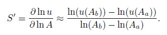 (24)
(24) To code the above formula, we can set $A_b =\alpha A_a +A_a $, where $\alpha $ is an increment that can be an arbitrarily small number. For the sensitivity analysis, $\alpha =10%$. By considering the relationship between $A_{b}$ and $A_{a}$ shown above, we have
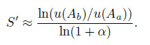 (25)
(25) When $u$ does not depend on the parameter $\alpha $, $S'=0$. If $u$ increases with an increase in $\alpha $, $S'$ is positive. On the contrary, $S'$ is negative if $u$ decreases with an increase in $\alpha $.
The drag force coefficient $C_{\mathrm D}$ and the secondary coefficient $K$ are chosen for the sensitivity analysis. Case I is selected as the reference condition. The bed friction coefficient is $C_\mathrm f =0.009$, the lateral dimensionless eddy viscosity is $\lambda =0.025$, the secondary flow coefficient is $| K |=0.03$, and the drag force coefficient is $C_\mathrm D a=0.255$.
First, we keep the other parameters unchanged and increase $C_\mathrm D a$ by 10% ($C_\mathrm D a=0.280 5) $. The results are plotted in Fig. 4 as a solid line. Then, the above process is repeated with an increase in the drag force coefficient ($K=0.033) $ of 10%, and the results are plotted in Fig. 4 by the dashed line.
|
|
| Fig. 4 Sensitivity analysis |
|
|
It can be seen from Fig. 4 that the sensitivity of $C_{\mathrm D}$ is quite close to the horizontal axis when $\eta >0$, which means that the drag force has little influence on the flow velocity in the non-vegetation zone. When $\eta <0$, the sensitivity parameter $S'$ is negative, and $u$ decreases by nearly 5% with a 10% increase in $C_{\mathrm D}$. It is clear that the drag force hinders the movement of water and this increases with a rise in $C_{\mathrm D}$, ensuring that the velocity decreases as a result. The secondary current coefficient mainly affects the velocity at the interface between the non-vegetation and vegetation zones, and extends through almost the whole non-vegetation zone. When $\eta <-0.05$, the change in the secondary current coefficient has almost no effect on the flow velocity, because the secondary current is impeded by the vegetation. When $-0.05<\eta <0$, $u $ decreases with an increase in $K$. When $\eta >0$, $u$ increases with an increase in $K$, and $u$ increases 5% at most in the non-vegetation zone with a 10% increase in $K$. This is consistent with the circulation of secondary currents.
The drag force coefficient varies along the vertical direction. Tang et al.[18] developed a model to calculate the vertically distributed coefficient,
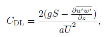 (26)
(26) where $-\overline {u'w'} $ means the Reynolds stress. Equation (26) indicates that the drag force coefficient is concerned with the Reynolds number. Considering that the present model is depth-averaged, Eq. (26) can be integrated along the $z$-axis,
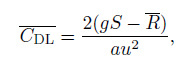 (27)
(27) where

The drag force coefficient may vary with different Reynolds numbers, and this feature should be considered if a more accurate velocity distribution is required.
6 Conclusions(i) This paper presents a two-dimensional solution for steady uniform flows in an open channel with partially covered vegetation across the channel using the singular perturbation method. The momentum exchange between vegetation and non-vegetation is considered by introducing a secondary flow coefficient. Based on the singular perturbed solution of the depth-averaged velocity, the Reynolds stress can be predicted. Comparisons with the experimental data show that consideration of the secondary flow term in the model significantly improves the prediction of velocity distributions, especially near the interface between the vegetation and non-vegetation zones. The singular perturbed method proves to be a useful tool for solving these nonlinear problems.
(ii) The effects of the secondary current intensity coefficient $K$ and the drag force coefficient $C_{\mathrm D}$ on the precision of the predictions are analyzed. The drag force coefficient mainly acts in the vegetation zone where the velocity is decreased by 5% with a 10% increase in $C_{\mathrm D}$. The secondary flow coefficient mainly influences the interface. The effect extends across almost the whole non-vegetation zone but decreases with an increasing distance from the interface.
| [1] | Li, R.M., & Shen, H.W Effect of tall vegetations on flow and sediment. Journal of the Hydraulics Division, 99(5), 793-814 (1973) |
| [2] | Tanino, Y, & Nepf, H.M Laboratory investigation of mean drag in a random array of rigid, emergent cylinders. Journal of Hydraulic Engineering, 134(1), 34-41 doi:10.1061/(ASCE)0733-9429(2008)134:1(34) (2008) |
| [3] | Wilson, C Flow resistance models for flexible submerged vegetation. Journal of Hydrology, 342(3), 213-222 (2007) |
| [4] | Liu, C., & Shen, Y.M Flow structure and sediment transport with impacts of aquatic vegetation. Journal of Hydrodynamics, Series B, 20(4), 461-468 doi:10.1016/S1001-6058(08)60081-5 (2008) |
| [5] | Chen, G., Huai, W.X., Han, J., & Zhao, M.D Flow structure in partially vegetated rectangular channels. Journal of Hydrodynamics, Series B, 22(4), 590-597 doi:10.1016/S1001-6058(09)60092-5 (2010) |
| [6] | Huai, W.X., Geng, C., Zeng, Y.H., & Yang, Z.H Analytical solutions for transverse distributions of streamwise velocity in turbulent flow in rectangular channel with partial vegetation. Applied Mathematics and Mechanics (English Edition), 32(4), 459-468 doi:10.1007/s10483-011-1430-6 (2011) |
| [7] | De Lima, A.C., & Izumi, N Linear stability analysis of open-channel shear flow generated by vegetation. Journal of Hydraulic Engineering, 140(3), 231-240 (2013) |
| [8] | Shimizu, Y., & Tsujimoto, T.N Numerical analysis of turbulent open-channel flow over a vegetation layer using a k-ε turbulence model. Journal of Hydroscience and Hydraulic Engineering, 11(2), 57-67 (1994) |
| [9] | VanProoijen, B.C., Battjes, J.A., & Uijttewaal, W.S Momentum exchange in straight uniform compound channel flow. Journal of Hydraulic Engineering, 131(3), 175-183 doi:10.1061/(ASCE)0733-9429(2005)131:3(175) (2005) |
| [10] | Tang, X., & Knight, D. Lateral depth-averaged velocity distributions and bed shear in rectangular compound channels. Journal of Hydraulic Engineering, 134(3), 1337-1342 (2008) |
| [11] | Rameshwaran, P., & Shiono, K Quasi two-dimensional model for straight overbank flows through emergent. Journal of Hydraulic Research, 45(3), 302-315 doi:10.1080/00221686.2007.9521765 (2007) |
| [12] | Shiono, K., & Knight, D.W Turbulent open-channel flows with variable depth across the channel. Journal of Fluid Mechanics, 222, 617-646 doi:10.1017/S0022112091001246 (1991) |
| [13] | Ervine, D.A., Babaeyan-Koopaei, K., & Sellin, R.H Two-dimensional solution for straight and meandering overbank flows. Journal of Hydraulic Engineering, 126(9), 653-669 doi:10.1061/(ASCE)0733-9429(2000)126:9(653) (2000) |
| [14] | Liu, C., Luo, X., Liu, X., & Yang, K Modeling depth-averaged velocity and bed shear stress in compound channels with emergent and submerged vegetation. Advances in Water Resources, 60, 148-159 doi:10.1016/j.advwatres.2013.08.002 (2013) |
| [15] | Ikeda, S., Izumi, N., & Ito, R Effects of pile dikes on flow retardation and sediment transport. Journal of Hydraulic Engineering, 117(11), 1459-1478 doi:10.1061/(ASCE)0733-9429(1991)117:11(1459) (1991) |
| [16] | White, B.L., & Nepf, H.M A vortex-based model of velocity and shear stress in a partially vegetated shallow channel. Water Resources Research, 44(1), W01412, 44(1), W01412 (2008) |
| [17] | Shiono, K., & Knight, D.W Turbulent open-channel flows with variable depth across the channel. Journal of Fluid Mechanics, 222, 617-646 doi:10.1017/S0022112091001246 (1991) |
| [18] | Tang, X., Knight, D.W., & Sterling, M Analytical model for streamwise velocity in vegetated channels. Proceedings of the ICE-Engineering and Computational Mechanics, 164(2), 91-102 (2011) |