 2016, Vol. 37
Shanghai University
Article Information
- Junbo CHENG
- Harten-Lax-van Leer-contact (HLLC) approximation Riemann solver with elastic waves for one-dimensional elasticplastic problems
- Applied Mathematics and Mechanics (English Edition), 2016, 37(11): 1517-1538.
- http://dx.doi.org/10.1007/s10483-016-2104-9
Article History
- Received Jan. 25, 2016
- Revised May. 6, 2016


This paper aims at the construction of a Harten-Lax-van Leer-contact (HLLC) approximate Riemann solver for one-dimensional elastic-plastic solid problems with the isotropic elasticplastic model initially developed by Wilkins[1] and the von Mises’ yielding condition and then builds a high-order cell-centered Lagrangian scheme. In Wilkins’ model, a perfectly elastic material is characterized by Hooke’s law in terms of an incremental strain resulting in an incremental stress, and the von Mises’ yielding criterion is used to describe the elastic limit.
The earliest simulation for elastic-plastic hydrodynamic equations with Wilkins’ model was developed by Wilkins[1], in which the equations of momentum and specific internal energy were discretized on a staggered grid, and the artificial viscosity was used to simulate moving shocks in order to damp spurious numerical oscillations.
Besides the staggered Lagrangian scheme, the Eulerian and cell-centered Lagrangian schemes have also been used to simulate elastic-plastic materials.
The Eulerian method[2-6] is suitable for the problems involving discontinuous waves and large deformations. However, most of Eulerian methods are just concerned with problems of hyper-elastic models for isotropic materials, and Eulerian methods for elastic-plastic materials with other constitutive models are seldom studied in the literature. In the papers for hyperelastic models[3-5], approximate and exact Riemann solvers were developed for elastic-plastic materials with hyper-elastic models, high-order finite-difference and finite-volume schemes were proposed, and good numerical results were obtained. In Ref. [6], the standard Prandtl-Reuss model was used, and a simple splitting method was introduced to discretize the governing equations with the strength material terms placed in the source terms.
Compared with the staggered Lagrangian schemes, the cell-centered Lagrangian schemes have their own advantages. For cell-centered Lagrangian schemes, it is not necessary to use artificial viscosity, and the schemes are conservative because the equation of total energy conservation, not the balance equation of the specific internal energy, is discretized. In the recent years, cell-centered Lagrangian schemes have attracted a lot of attention (see, for example, Refs. [7]-[10]), and they have been applied not only to the hyper-elastic models but also to the hypo-elastic models (see Refs. [7]-[10]). In these papers, the nodal Riemann solver was used in the construction of cell-centered Lagrangian schemes, but the structure of the associated Riemann solution was not taken into account.
Some authors have used the structure of the Riemann solution to construct Riemann solvers for the governing equations of hypo-elastic models (see Refs. [11]-[13] for example). Gavrilyuk et al.[11] analyzed the structure of the Riemann solution to construct a Riemann solver for the linear elastic system of hyperbolic non-conservative models for transverse waves. In addition, the elastic energy was included in the total energy[11], and an extra evolution equation was added in order to make the elastic transformations reversible in the absence of shock waves. Despr´ es[12] built a shock solution to a non-conservative system of hypo-elasticity models and found that a sonic point is necessary to construct a compression solution that begins at a constrained compressed state. Cheng et al.[13] analyzed the wave structures of one-dimensional elasticplastic flows and developed a two-rarefaction Riemann solver with elastic waves (TRRSE) and built the second-order and third-order cell-centered Lagrangian schemes based on the TRRSE. Numerical results evaluated by the TRRSE show the effectiveness of TRRSE, but the iteration method used in the TRRSE means that the approximation Riemann solver is a little expensive.
The aim of the current paper is to extend the HLLC approximate Riemann solvers[14] from pure fluids to elastic-plastic flows. First, we construct the HLLC Riemann solvers with elastic wave (HLLCE) for a non-conservative system with Wilkins’ model and von Mises’ yielding criterion. Finally, we use the constructed HLLCE to evaluate the numerical flux in high-order cell-centered Lagrangian schemes and propose high-order cell-centered Lagrangian schemes for one-dimensional elastic-plastic problems. In order to keep our schemes positivity-preserving, the time step is limited in order to make the density and internal energy positive during the simulation of these problems.
The rest of this paper is organized as follows. In Section 2, we introduce the governing equations to be studied. In Section 3, we construct the HLLCE. We develop high-order cell-centered Lagrangian schemes for a non-conservative system of elastic plasticity in Section 4. In Section 5, we show how to limit the time step to keep our schemes positivity-preserving. A number of numerical examples are presented in Section 6 to validate the schemes. Finally, conclusions are given.
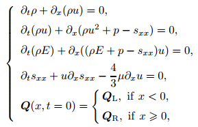
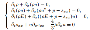
2 Governing equations 2.1 Equations of motionThe equations for a continuous one-dimensional homogeneous solid in the differential form read as

|
(1) |
Here,
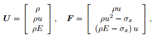
|
(2) |
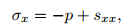
where ρ is the density, u is the velocity in the x-direction, E is the total energy per unit volume, 
|
(3) |
where p is the hydrostatic pressure which is a function of the density and the specific internal energy, and sxx is the deviatoric stress. We remark here that the elastic energy is not included in the total energy in this paper. The exclusion of the elastic energy is usual for practical engineering problems (see Ref. [9]) and is different from that in Ref. [11].
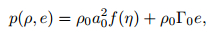
In this paper, we consider the Mie-Grüneisen equation of state (EOS),
|
(4) |
where 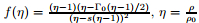
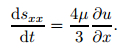
Hooke’s law is used here to describe the relationship between the stress and the strain,
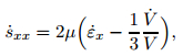
|
(5) |
where μ is the shear modulus, V is the volume, and the dot means the material time derivative,
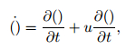
|
(6) |
and

|
(7) |

|
(8) |
Using (7) and (8), we can rewrite (5) as
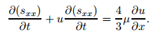
|
(9) |
The von Mises’ yielding condition is used here to describe the elastic limit. In one spatial dimension, the von Mises’ yielding criterion is given by
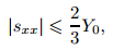
|
(10) |
where Y0 is the yield strength of the material in simple tension.
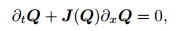
3 HLLCEThe Riemann problem for the one-dimensional time dependent elastic-plastic equations reads as follows:
|
(11) |
where Q = (ρ, ρu, ρE, sxx)T.
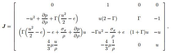
3.1 Analysis of Jabocian matrixFor the Mie-Grüneisen EOS, the problem (11) can be written as
|
(12) |
where
|
(13) |
where 
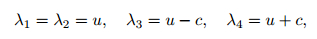
The eigenvalues of the coefficient matrix A(W) are given by
|
(14) |
where
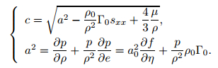
|
(15) |
The corresponding right eigenvectors are
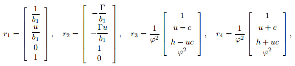
|
(16) |
where
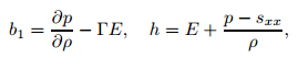
|
(1) |
and
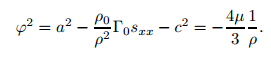
|
(17) |
The structure of the solution to the Riemann problem (12) in the xt-plane is depicted in Fig. 1. It consists of three waves emanating from the origin, each one for each eigenvalue λi given in (14). λ1 and λ2 correspond to the contact wave, while λ3 and λ4 correspond to the leftgoing and right-going rarefaction waves, respectively. These three waves separate four constant states. From left to right, these states are WL (left data state), WL* (between the λ1-wave and the λ3-wave), WR* (between the λ1-wave and the λ4-wave), and WR (right data state).

|
| Fig. 1 Structure of Riemann problem |
|
|
Using the eigenvectors (16), for the λ1-wave, we have
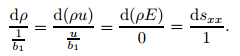
|
(18) |
From the above equations, we can easily deduce that
|
(19) |
which means

|
(20) |
and
|
(21) |
where ()L* and ()R* denote () in the regions of WL* and WR*, respectively. Here, we do not show the details of the derivation for simplicity of presentation.
Using the eigenvectors (16), for the λ2-wave, we have
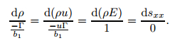
|
(22) |
From the above equations, we can easily deduce that
|
(23) |
which means

|
(24) |
|
(25) |
where ()L* and ()R* denote () in the regions of WL* and WR*, respectively.
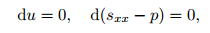
Thanks to (25), one gets
|
(26) |
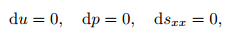
At last, for the λ1 and λ2 waves, one can find that the following two equations always hold:
|
(27) |
Consider Fig. 2, in which the whole of the wave structure arising from the solution of the Riemann problem is contained in the control volume [xL, xR] × [0, T], that is,

|
| Fig. 2 Control volume [xL, xR] × [0, T] on xt-plane, where sL and sR are slowest and fastest signal velocities arising from solution of Riemann problem |
|
|
|
(2) |
where sL and sR are the slowest and fastest signal velocities perturbing the initial data states UL and UR, respectively, and T is the chosen time. The integral form of the conservation laws in (1) in the control volume [xL, xR] × [0, T] reads

|
(28) |
Using the method for the Harten-Lax-van Leer (HLL) approximate Riemann solver introduced in Ref. [14], one can get
|
(3) |
Dividing the above equation by T(sR − sL) gives
|
(29) |
Therefore, the integral average of the exact solution of the Riemann problem between the slowest and fastest signals at the time T is a known constant. Provided that the signal speeds sL and sR are known, such a constant is the right hand side of (29), and we denote it by
|
(30) |
Consider Fig. 2, in which the complete structure of the solution of the Riemann problem is contained in a sufficiently large control volume [xL, xR] × [0, T]. Now, in addition to the slowest and fastest signal speeds sL and sR, we include a middle wave of the speed s*. Evaluation of the integral form of the conservation laws in the control volume reproduces the result of equation (29), even if variations of the integrand across the wave of the speed s* are allowed. By splitting the left-hand side of integral (29) into two terms, we obtain
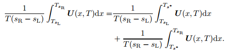
|
(31) |
Define the integral averages
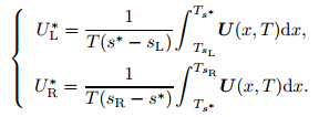
|
(32) |
Thanks to (29), (30), (31), and (32), one can have
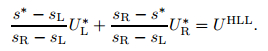
|
(33) |
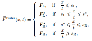
The HLLCE is given as follows:
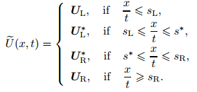
|
(34) |
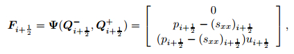
A corresponding HLLCE numerical flux in the Eulerian framework is defined as
|
(35) |
and a corresponding HLLCE numerical flux in the Lagrangian framework is defined as

|
(36) |
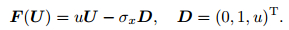
where fL*= Ψ(UL*), fR* = Ψ(UR*), and Ψ = (0, −σx, −σxu)T.
Applying Rankine-Hugoniot conditions across each of the waves of speeds sL, s*, and sR, we obtain
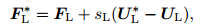
|
(37) |
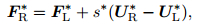
|
(38) |
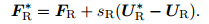
|
(39) |
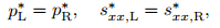
We need to evaluate the solutions for the two unknown intermediate fluxes FL* and FR*. From (37)-(39), we can see that it is not sufficient to find solutions for the two intermediate state vectors UL* and UR*. There are more unknowns than equations, and some extra conditions need to be imposed in order to solve the algebraic problem. Obvious conditions to impose are those satisfied by (27). For the normal velocity and the normal stress, we have
|
(40) |
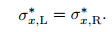
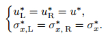
In addition, it is entirely justified and convenient to set

|
(41) |
Thus, if an estimate for s* is known, the normal velocity u* in the star region is known. Besides, we can note that
|
(42) |
Assuming that the wave speeds sL and sR are known, substituting (42) into (37) and (39) and then performing algebraic manipulations of the first and second components of (37) and (39), we can get the following solutions for the normal stress in the two star regions:
|
(43) |
|
(44) |
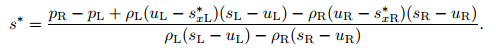
From the second equation of (40), we can get the formulation of s* as follows:
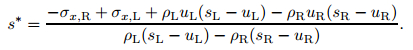
|
(45) |
Thus, we only need to provide estimates for sL and sR. We can evaluate all the values of UL* and UR*. However, there is one problem that we need to solve. We need to decide whether the deviatoric stresses in the central regions are over the elastic limit or not. If yes, we have to use the von Mises’ yielding condition to modify sxx. However, first, we need to evaluate the values of sxx in the central regions without considering von Mises’ yielding condition. In the following, we show how to evaluate sxx.
First, we evaluate the values of p in the central region, pL* and pR*. Just like the formulations of σx in (43) and (44), we define
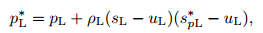
|
(46) |
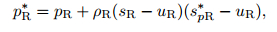
|
(47) |
where spL* and spR* are unknown variables.
According to sxx = σx + p, adding (43) to (46) yields
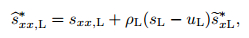
|
(48) |
where
|
(49) |
Using the same method, adding (44) to (47) yields
|
(50) |
where

|
(51) |
We assume that

|
(52) |
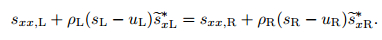
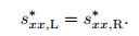
This assumption is not the loss of generality because the equality always holds for pure fluids. According to sxx = σx + p, thanks to the second equation of (40), we can get
|
(53) |
Thanks to (48), (50), and the above equation, we can get
|
(54) |
We assume that

|
(55) |
The equality always holds for pure fluids. Therefore, this assumption is not the loss of generality.
Thanks to (49) and (51), according to (55), we can get
|
(56) |
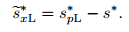
Combining (56) with (54) and performing algebraic manipulations, one gets

|
(57) |
After getting the value of 


Case 1 If 

Case 2 If 

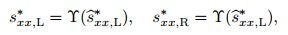
|
(58) |
where the function
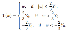
|
(59) |
and w is a scalar.
Because 
|
(60) |
Then, we use (48) and (50) to evaluate sxL* and sxR*, respectively,
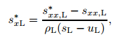
|
(61) |
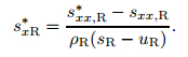
|
(62) |
Obviously,

|
(4) |
Based on (49) and (51), we define
|
(63) |
According to (60) and the second equation of (40), we can get

|
(5) |
This shows that the previous assumption in (52) is applicative even if the deviatoric stresses are modified because they are over the elastic limit.
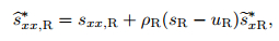
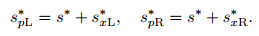
According to the above equation and (63), from (46) and (47), we can get

|
(64) |
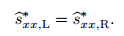
After performing algebraic manipulations of the above equations, we can obtain
|
(65) |
Combining the above equation with (63), we can get the values of spL* and spR*. Then, we use (46) and (47) to evaluate pL* and pR*. At last, we can get
|
(66) |
As for the wave speeds sL and sR, we use the simple estimates,

|
(67) |
Here, we present all procedures of HLLCE.
Step 1 Evaluate
|
(68) |
Step 2 Evaluate
|
(69) |
|
(70) |
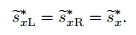
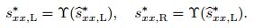
Step 3 Use the von Mises’ yielding condition to modify
|
(6) |
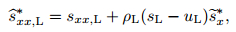
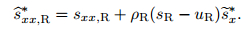
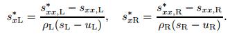
Step 4 Re-evaluate sxL* and sxR*,
|
(7) |
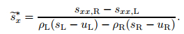
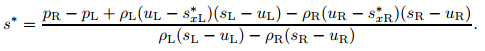
Step 5 Evaluate s*,
|
(8) |
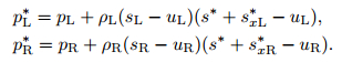
Step 6 Evaluate pL* and pR*,
|
(9) |
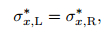
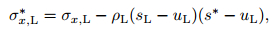
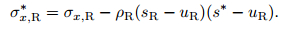
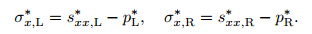
Step 7 Evaluate σx, L* and σx, R*,
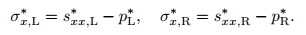
|
(10) |
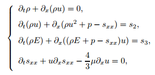
Here, we consider the following governing equations with Wilkins’ model:
|
(71) |
under appropriate initial and boundary conditions. Moreover, for a Lagrangian scheme, the governing equations also include the equation for moving the coordinates at the vertex of the mesh,
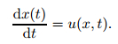
|
(72) |
The spatial domain is discretized into N computational cells 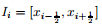

|
(73) |
The semi-discrete finite volume scheme of the conservative equations (1) in the cell Ii is written as
|
(74) |
where
|
(75) |


The first step for establishing the high-order scheme is to determine the flux 

The reconstruction for (71) is carried out in local characteristic variables. We first transform the conservative variables to the characteristic variables and then apply the third-order weighted essentially non-oscillatory (WENO) reconstruction method to reconstruct each component of the characteristic variables. The final values are obtained by transforming back to the conservative variables.
Let us denote by Ji the Jacobian (13) in Ii, and denote by R (column vector) and L (row vector) the right and left eigenvectors of Ji, respectively. We transform Q to the characteristic variables
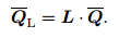
|
(76) |
From QL, we perform the procedure of the third-order WENO reconstruction at the left and right cell interfaces of Ii. At last, all these point-wise values are projected back to the component space. Now, we obtain the values of Q at the left side and the right side of the cell’s boundary,
We solve the following Riemann problem:
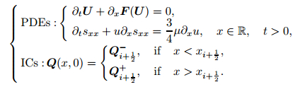
|
(77) |
We denote the similarity solution of (77) by D(0)(x/t). Then, the Godunov value of Q is given by
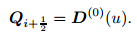
|
(78) |
Because the grid moves at the fluid speed, the Godunov value of Q should be the value of Q on the contact discontinuity of the Riemann solution. We evaluate them by the following two steps.
Step A1 Evaluate the state in the star region in the Riemann solution. First, given the initial value of Q, we get the value of W. Then, we use the TRRSE to evaluate the state in the star region in the Riemann solution. At last, we can get
|
(79) |
where WL* = (ρL*, uL*, pL, sxx, L*), and WR* = (ρR*, uR*, pR*, sxx, R*).
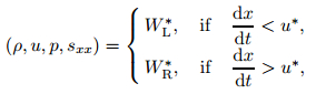
Step A2 Define the Godunov values of ρ, u, p, and sxx: ρ*, u*, p*, and sxx*,
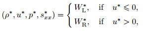
|
(80) |
where WL* = (ρL*, uL*, pL, sxx, L*), and WR* = (ρR*, uR*, pR*, sxx, R*).
Remark 1 Because the stress and velocity are constant in the star region of the Riemann solution, and the numerical flux is just involved with the stress and velocity, it does not affect the final results to choose the left or right state as the Godunov values.
After obtaining the Godunov values of ρ, u, p, and sxx, we can use (75) to evaluate the numerical flux of the conservative equation (1).
4.1.3 Spatial discretization of constitutive equationIn the Lagrangian frame, the equation of the constitute model (9) can be written as
|
(81) |
For the cell-centered Lagrangian scheme, the geometrical conservation law is very important, that is, (8) should be satisfied. In the one-dimensional case, the volume of the cell Ii is evaluated by
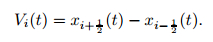
|
(82) |
Taking the material derivative on both sides of (82), we have
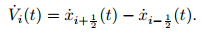
|
(83) |
By virtue of (72), (83) becomes
|
(84) |
Combining (82) and (84), one gets
|
(85) |
Therefore, using (8), we can discretize 
|
(86) |
Thanks to (86), the semi-discrete formulation for (81) in the cell Ii has the following form:
|
(87) |
where 
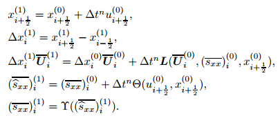
The time marching for the semi-discrete scheme (72), (74), (87), and von Mises’ yielding condition is implemented by the total variation diminishing (TVD)-type Runge-Kutta method. Since the grid changes with the time advancing in the Lagrangian simulation, the velocity, the position of each vertex, and the cell size need to be updated at each Runge-Kutta stage. Thus, the form of the third-order Runge-Kutta method in the Lagrangian schemes reads as follows:
Step 1
|
(11) |
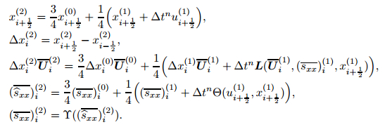
Step 2
|
(12) |
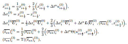
Step 3
|
(13) |
where 

In the above formulations, L and Θ are the numerical spatial operators representing the right hands of the scheme (74) and the scheme (87), respectively, and the variables with the superscripts n and n+1 denote the values of the corresponding variables at the nth and (n+1)th time steps, respectively.
5 Positivity-preserving time stepIn this section, we define the positivity-preserving time step, which not only keeps our scheme stable but also makes our scheme positivity-preserving. The concept of positivity-preserving is very important in practical simulations, and there are many high-order schemes about positivity-preserving, such as high-order finite volume methods of positivity-preserving[16], high-order discontinuous Galerkin methods of positivity-preserving[17-18], high-order ENO Lagrangian schemes of positivity-preserving[19], and a high-order cell-centered Lagrangian scheme of positivity-preserving for one-dimensional elastic-plastic flows[13].
In Ref. [13], the TRRSE was used to evaluate the Godunov values at the interface. Here, the HLLCE is used, but the procedure for deducing the positivity-preserving scheme is the same as that in Ref. [13]. In order to simplify the presentation, we do not show the details. If one is interested in it, please refer to Ref. [13].
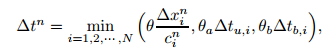
Just like Ref. [13], the time step Δtn of the scheme is given as
|
(14) |
where θ = 0.45, θa = θb = 0.9, and cin is the sound speed of solid in the cell i at the time tn,
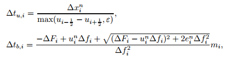
|
(15) |
mi = Δxinρin, 
In this section, we test the proposed scheme with different problems to demonstrate the capability of the scheme in capturing elastic-plastic waves. Moreover, we use different grids to test the convergence of the present scheme.
For simplicity, we denote by CLk-HLLCE and CLk-TRRSE the kth-order cell-centered Lagrangian scheme with our developed HLLCE and the kth-order cell-centered Lagrangian scheme with the TRRSE introduced in Ref. [13], respectively, where k = 1, 3.
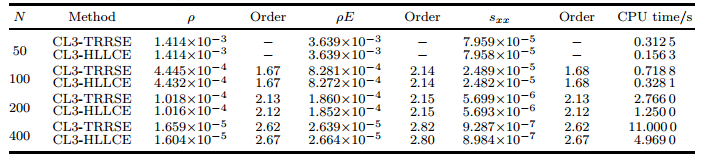
6.1 Accuracy testWe use smooth manufactured solutions to test the accuracy of the third-order scheme. The method of manufactured solutions is a very simple process, which was introduced in detail in Refs. [20] and [21]. We consider the following compressible equations with source terms:
|
(88) |
where
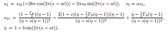
|
(16) |
and a, b, and s0 are constant parameters.
The smooth manufactured solutions of the above equations with the source terms are

|
(17) |
where e0 is the constant internal energy.
The computational domain is [0, 1], and a periodic boundary condition is used. The EOS is given by the Mie-Grüneisen model with the parameters ρ0 = 8 930 kg/m3, a0 = 3 940 m/s, Γ0 = 2, and s = 1.49. The constitutive model is characterized by the following parameters: the shear module μ = 4.5× 10¹⁰ Pa and the yield strength Y0 = 9× 10¹⁰ Pa. The initial conditions are given as

|
(18) |
where a = 10 000 m/s, b = 0.2, s0 = 60 × 106 Pa, and e0 = 0.1.
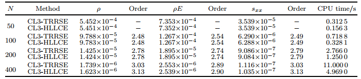
We use CL3-TRRSE and our CL3-HLLCE to numerically solve the problem. Because there are some source terms in this problem, we have to compute 

The CPU time and L1- and L∞-norm errors at the output time t = 1 are shown in Tables 1 and 2, from which we see that our CL3-HLLCE achieves the desired accuracy, and the L1- and L∞-norm errors of CL3-HLLCE are almost equal to these of CL3-TRRSE. However, the CPU time costed by CL3-HLLCE is about half of that by CL3-TRRSE. This shows that CL3-HLLCE is more efficient than CL3-TRRSE.
 |
 |
This piston problem introduced in Ref. [22] is concerned with a piece of copper with the following initial setting: the length of copper is 1 m, the initial density ρ0 = 8 930 kg/m3, the initial pressure p0 = 105 Pa, and the initial velocity is zero. The EOS for copper is given by the Mie-Grüneisen model with the parameters ρ0 = 8 930 kg/m3, a0 = 3 940 m/s, Γ0 = 2, and s = 1.49. The constitutive model is characterized by the following parameters: the shear module μ = 4.5× 10¹⁰ Pa and the yield strength Y0 = 9× 10⁷ Pa. The left boundary condition is a velocity boundary condition given by vpiston = 20 m/s, whereas on the right boundary of the computation domain, the wall boundary condition is implemented.
In order to empirically test the convergence of our scheme, we use CL3-HLLE to evaluate the problem with 100, 200, and 400 cells. The stopping time is t = 150 μs. The numerical results with different Δx are shown in Figs. 3 and 4, from which we can see that the numerical solution converges to the exact solution. Obviously, the current scheme well captures the leading elastic shock wave and the followed plastic shock wave. Note that there is no numerical oscillation near the shock waves.

|
| Fig. 3 Density and velocity versus x at time t = 150 μs in piston problem |
|
|

|
| Fig. 4 Piston problem, pressure, and sxx versus x at time t = 150 μs |
|
|
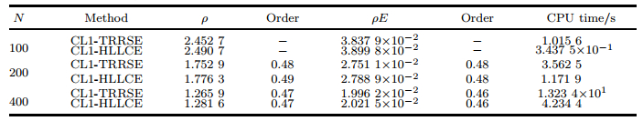
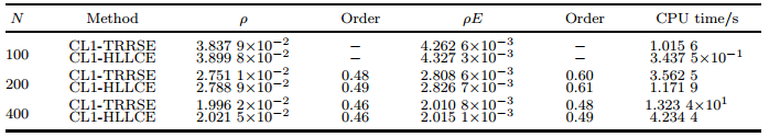
In order to check the ability of our developed HLLCE, we use CL1-HLLCE and CL1-TRRSE to simulate this problem. The comparison between two schemes is found in Fig. 5. We can see that the numerical results of CL1-HLLCE agree very well with those computed by CL1- TRRSE, which shows that the resolution of CL1-HLLCE is almost the same as that of CL1- TRRSE around shock waves. Beside, in Tables 3 and 4, one can find that two schemes have almost the same resolution for shock waves, but obviously, CL1-HLLCE is more efficient because the CPU time costed by CL1-HLLCE is less than that by CL1-TRRSE. Moreover, Fig. 6 shows that CL1-HLLCE is more efficient than CL1-TRRSE, which is understandable because the iteration procedure is not used in the HLLCE, while it is used in the TRRSE.

|
| Fig. 5 Comparison of density between numerical result of CL1-HLLCE and that computed by CL1-TRRSE using 100 cells in piston problem |
|
|
 |
 |

|
| Fig. 6 CPU time versus L1 and L∞ errors of CL1-HLLCE and CL1-TRRSE in piston problem |
|
|
This problem, originally introduced by Wilkins[1], is used here to show the ability of our scheme to compute rarefaction waves. This problem describes a moving aluminium plate striking on another aluminium plate. The EOS for aluminium is the Mie-Grüneisen model with the parameters ρ0 = 2785 kg/m3, a0 = 5328 m/s, Γ0 = 2, and s = 1.338. The constitutive model is characterized by the following parameters: the shear module μ = 2.76 × 10¹⁰ Pa and the yield strength Y0 = 3 × 10⁸ Pa. The initial conditions of this problem are

|
(89) |
We use 200, 400, and 800 cells to simulate the problem up to 5×10⁻⁶s with the free boundary condition on the left boundary and the wall boundary condition on the right boundary. The computed results are presented in Figs. 7-10. The reference solutions (solid lines in all the figures) are computed by CL3-HLLE using 4 000 cells.

|
| Fig. 7 Density versus x at time t = 5 μs in Wilkins’ problem with Mie-Grüneisen EOS, where right figure is close-up of region around head of right-facing elastic rarefaction wave |
|
|

|
| Fig. 8 Velocity versus x at time t = 5 μs in Wilkins’ problem with Mie-Grüneisen EOS, where right figure is close-up of region around head of right-facing elastic rarefaction wave |
|
|

|
| Fig. 9 Pressure versus x at time t = 5 μs in Wilkins’ problem with Mie-Grüneisen EOS, where right figure is close-up of region around right-facing elastic shock wave |
|
|

|
| Fig. 10 sxx versus x at time t = 5 μs in Wilkins’ problem with Mie-Grüneisen EOS, where right figure is close-up of region around head of right-facing elastic rarefaction wave |
|
|
From Figs. 7-10, we can observe that the numerical solution converges to the reference one. Obviously, the elastic and plastic right-facing shocks and the reflected elastic and plastic rarefaction waves are well resolved, and the numerical results are in good agreement with those given in Ref. [9].
We also compare the numerical results of CL1-HLLCE with those of CL1-TRRSE in Ref. [13] in Fig. 11. In Fig. 11, we can see that

|
| Fig. 11 Comparison of density between numerical results of CL1-HLLCE and those computed by CL1-TRRSE using 100 cells in Wilkins’ problem with Mie-Grüneisen EOS and close-up of regions around rarefaction waves and shock waves |
|
|
(i) The TRRSE has a little higher resolution in resolving the rarefaction wave than the HLLCE because the TRRSE is exact in resolving the rarefaction wave, while the HLLCE is approximate for the the rarefaction wave.
(ii) The numerical results computed by CL1-HLLCE agree very well with those computed by CL1-TRRSE for the elastic shock wave.
7 ConclusionsIn this paper, we develop the HLLCE for one-dimensional elastic-plastic materials with the Mie-Grüneisen EOS and Wilkins’ constitutive model, where the von Mises’ yielding criterion is used. Then, based on the HLLCE, we use the third-order finite volume scheme to discretize the equations of one-dimensional elastic-plastic materials in the Lagrangian framework. At the cell interfaces, the HLLCE constructed in this paper is used to evaluate the Godunov values of the density, pressure, velocity, and stress. Besides, the time step is limited to keep this third-order scheme positivity-preserving for one-dimensional elastic-plastic fluid problems. Numerical simulation of the smooth problems with Wilkins’ constitutive model shows that our third-order scheme achieves the third-order accuracy. We also use the high-order scheme to simulate the piston and Wilkins’ problems. The numerical tests demonstrate the convergence of our scheme, and the numerical results computed by the current scheme are in good agreement with those obtained by other authors. Moreover, although the present scheme based on the HLLCE performs a little worse than the same-order scheme based on the TRRSE in solving rarefaction waves, for shock waves, the numerical results of the third-order scheme based on the HLLCE agree very well with those computed by the third-order scheme based on the TRRSE. Moreover, the scheme based on HLLCE performs more efficient than the scheme based on the TRRSE.
In the near future, we shall build multi-dimensional Riemann solvers based on the current one-dimensional Riemann solver for multi-dimensional elastic-plastic problems and develop a high-order cell-centered Lagrangian scheme for multi-dimensional elastic-plastic flows.
| [1] | Wilkins, M. L. Methods in Computational Physics, Vol. 3, 1964, Chapter Calculation of Elastic-Plastic Flow. Academic Press, New York, 211-263 (1964) |
| [2] | Hill, D. J., Pullin, D., Ortiz, M., & Meiron, D. An Eulerian hybrid WENO centered-difference solver for elastic-plastic solids. Journal of Computational Physics, 229, 9053-9072 (2010) doi:10.1016/j.jcp.2010.08.020 |
| [3] | Miller, G. H., & Collela, P. A high-order Eulerian Godunov method for elastic-plastic flow in solids. Journal of Computational Physics, 167, 131-176 (2001) doi:10.1006/jcph.2000.6665 |
| [4] | Trangenstein, J. A., & Collela, P. A high-order Godunov method for modeling finite deformation in elastic-plastic solids. Communications on Pure and Applied Mathematics, 44, 41-100 (1991) doi:10.1002/(ISSN)1097-0312 |
| [5] | Barton, P. T., Drikakis, D., Romenski, E., & Titarev, V. A. Exact and approximate solutions of Riemann problems in non-linear elasticity. Journal of Computational Physics, 228, 7046-7068 (2009) doi:10.1016/j.jcp.2009.06.014 |
| [6] | Menshov, I., Mischenko, A., and Serezhkin, A. An Eulerian Godunov-type scheme for calculation of the elastic-plastic flow equations with moving grids. The 6th European Congress on Computational Methods in Applied Sciences and Engineering 2012(ECCOMAS 2012), Vienna University of Technology, Vienna, 4099-4118(2012) |
| [7] | Burton, D. E., Carney, T. C., Morgan, N. R., Sambasivan, S. K., & Shashkov, M. J. A cellcentered Lagrangian Godunov-like method for solid dynamics. Computers and Fluids, 83, 33-47 (2013) doi:10.1016/j.compfluid.2012.09.008 |
| [8] | Kluth, G., & Desprès, B. Discretization of hyperelasticity on unstructured mesh with a cellcentered Lagrangian scheme. Journal of Computational Physics, 229, 9092-9118 (2010) doi:10.1016/j.jcp.2010.08.024 |
| [9] | Maire, P. H., Abgrall, R., Breil, J., Loubère, R., & Rebourcet, B. A nominally second-order cellcentered Lagrangian scheme for simulating elastic-plastic flows on two-dimensional unstructured grids. Journal of Computational Physics, 235, 626-665 (2013) doi:10.1016/j.jcp.2012.10.017 |
| [10] | Sambasivan, S. K., Loubere, R., and Shashkov, M. J. A finite volume Lagrangian cell-centered mimetic approach for computing elasto-plastic deformation of solids in general unstructed grids.The 6th European Congress on Computational Methods in Applied Sciences and Engineering 2012(ECCOMAS 2012), Vienna University of Technology, Vienna (2012) |
| [11] | Gavrilyuk, S. L., Favrie, N., & Saurel, R. Modeling wave dynamics of compressible elastic materials. Journal of Computational Physics, 227, 2941-2969 (2008) doi:10.1016/j.jcp.2007.11.030 |
| [12] | Desprès, B. A geometrical approach to non-conservative shocks elastoplastic shocks. Archive for Rational Mechanics and Analysis, 186, 275-308 (2007) doi:10.1007/s00205-007-0083-3 |
| [13] | Cheng, J. B., Eleuterio, F. T., Song, J., Ming, Y., & Tang, W. J. A high-order cell-centered Lagrangian scheme for one-dimensional elastic-plastic problems. Computer and Fluids, 122, 136-152 (2015) doi:10.1016/j.compfluid.2015.08.029 |
| [14] | Eleuterio, F. T. Riemann Solvers and Numerical Methods for Fluid Dynamics. Springer, London/New York (1997) |
| [15] | Jiang, G. S., & Shu, C. W. Efficient implementation of weighted ENO schemes. Journal of Computational Physics, 126, 202-228 (1996) doi:10.1006/jcph.1996.0130 |
| [16] | Perthame, B., & Shu, C. W. On positivity preserving finite volume schemes for Euler equations. Numerische Mathematik, 73, 119-130 (1996) doi:10.1007/s002110050187 |
| [17] | Zhang, X., & Shu, C. W. On positivity preserving high order discontinuous Galerkin schemes for compressible Euler equations on rectangular meshes. Journal of Computational Physics, 229, 8918-8934 (2010) doi:10.1016/j.jcp.2010.08.016 |
| [18] | Zhang, X., & Shu, C. W. Positivity-preserving high order discontinuous Galerkin schemes for compressible Euler equations with source terms. Journal of Computational Physics, 230, 1238-1248 (2011) doi:10.1016/j.jcp.2010.10.036 |
| [19] | Cheng, J., & Shu, C. W. Positivity-preserving Lagrangian scheme for multi-material compressible flow. Journal of Computational Physics, 257, 143-168 (2014) doi:10.1016/j.jcp.2013.09.047 |
| [20] | Roache, P. J. Code verification by the method of manufactured solutions. Journal of Fluids Engineering, 124, 4-10 (2002) doi:10.1115/1.1436090 |
| [21] | Salari, K. and Knupp, P. Code Verification by the Method of Manufactured Solutions, Sandia Report, SAND2000-1444, Sandia National Laboratories, Albuquerque (2000) |
| [22] | Maire, P. H., & Breil, J. A second-order cell-centered Lagrangian scheme for two-dimensional compressible flow problems. International Journal for Numerical Methods in Fluids, 56, 1417-1423 (2008) doi:10.1002/(ISSN)1097-0363 |