 2019, Vol. 40
Shanghai University
Article Information
- Zeyu LIU, Yantao YANG, Qingdong CAI
- Neural network as a function approximator and its application in solving differential equations
- Applied Mathematics and Mechanics (English Edition), 2019, 40(2): 237-248.
- http://dx.doi.org/10.1007/s10483-019-2429-8
Article History
- Received Sep. 5, 2018
- Revised Oct. 25, 2018


2. Department of Mechanics and Engineering Science, College of Engineering, Peking University, Beijing 100871, China;
3. Center for Applied Physics and Technology, College of Engineering, Peking University, Beijing 100871, China
An artificial neural network (ANN) is a computing system inspired by the complex biological neural networks (NNs) constituting animal brains[1]. The original purpose of constructing an ANN was to mimic the problem solving process that occurs in the human brain. However, due to the complexity of the human brain, this goal has not been achieved at the current stage, and it is believed that the gap is still difficult to bridge[2]. However, impressive achievements have been made in a variety of tasks like image recognition[3], natural language processing[4], cognitive science[5], and genomics[6].
NNs consist of artificial neurons (simplified biological neurons) and connections (also called edges) of artificial neurons (simplified synapses). The output of each neuron is a non-linear bounded function of the weighted sum of its inputs. The neurons are usually arranged into layers, where connections are established between layers.
The NN was introduced as computing machine in the 1940s[7], and Rosenblatt[8] later introduced the first model of supervised learning based on a single layer NN with a single neuron. Rosenblatt[9] also presented an algorithm to adjust the free parameters in a learning procedure, and proved the convergence of the algorithm, which is now known as the perceptron convergence theorem. Multilayer NNs were introduced naturally after the single layer case. However, due to the difficulty of properly training a multilayer NN[10], little progress has been made.
In the mid-70s, the development of hardware and the backpropagation algorithm[11] renewed the interest in the NNs. One important technique is the automatic differentiation (AD). For closed-form expressions, the AD is a numerical evaluation of symbolic differentiation. However, the AD is useful not only for closed-form expressions, but also for any computing program constructed from elementary mathematical operations[12]. The AD calculates the derivative of a function defined by a computer program by performing a non-standard interpretation of the program, and the interpretation replaces the domain of the variables and redefines the semantic of the operators. The AD algorithm calculates derivatives using the chain rule from the differential calculus[13]. Moreover, the AD is of much greater significance than a mathematically rigorous description of the backpropagation algorithm, i.e., it provides a universal method for calculating derivatives. Thus, machine-learning researchers do not need to manually calculate derivatives and code the complicated formulae that are prone to errors.
Recently, a numerical solver combining NNs with the AD was proposed for solving differential equations[14]. When solving a differential equation, one seeks a function in the space and time which satisfies the differential equation within the domain, and any boundary and initial conditions. In practice, one can define a loss function associated with some trial functions using the residual of the differential equations and the boundary/initial conditions, and the solution can be found by minimizing the loss function. There are many networks from which to choose, such as the Legendre NN[15], the Chebyshev NN[16], the deep ANN[17], and radial basis function networks[18-19]. In order to construct the loss function from the residual, one needs to evaluate the derivative of the output layer with respect to the input layer, which can be done using the AD technique. Such a strategy of applying a deep NN to solving a differential equation is highly feasible. Furthermore, the order of the differential equation is no longer a limitation, while traditional methods are usually limited to second-order systems.
In this study, we first discuss our systematic research on the use of NNs for the function approximation. Then, the method will be used to solve several differential equations. The solver is constructed using TENSORFLOW[20], which provides application programming interfaces (APIs) and a parallelism framework. In particular, we will demonstrate the method by solving the heat equation in a two-dimensional cavity. The paper is then concluded with discussion and future perspectives.
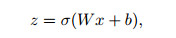
2 NN as a function approximatorEach layer of a fully connected NN can be described as
|
(1) |
where x is the input vector, z is the output vector, W is the weight matrix, b is the bias vector, and σ(x) is an activation function. In the rest of this paper, we denote the closed unit cube in the n-dimensional space as In. Therefore, all continuous functions defined on In are denoted as C(In). Similarly, all functions defined on In, which are Lp integrable, are denoted as Lp(In). Functions in the form of Eq. (1) are dense in C(In) if the activation function σ is monotonic sigmoidal[21], which means that any continuous function defined in a finite domain can be accurately approximated with a fully connected NN. It was previously proven[22-24] that, given different assumptions on the activation function σ, functions of the above form are dense in other function spaces, e.g., 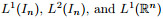
One important property of an NN function approximator is that it works well for interpolation and fitting. Traditional interpolation methods and fitting methods are quite different. The NN provides a unified framework of processing input and output data in order to reconstruct a map between them. With a small set of accurate data, an NN function approximator interpolates the given data, and with a large set of noisy data, the NN function approximator fits the given data.
An NN function approximator is constructed in a supervised learning process. The training set 

|
(2) |
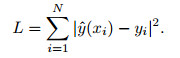
The training process requires the loss function minimized with respect to the weights and biases in each network layer. The gradient descent method, which is robust and fairly easy to code, converges fast enough for this optimization problem.
To demonstrate the interpolation property of an NN function approximator, we take f(x)=sin x + sin (1.7x) as an example. The interpolation points are selected uniformly on the interval [-2, 4] with the equal distance 0.5 between two neighboring points. For comparison, the spline interpolation is also applied to the same interpolation points. Figure 1 shows the function interpolated with an NN function approximator and cubic spline interpolation with error, which is defined as 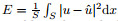

|
| Fig. 1 Interpolation by the NN and cubic spline (color online) |
|
|

|
| Fig. 2 First-order derivative of interpolated NN and cubic spline (color online) |
|
|

|
| Fig. 3 Second-order derivative of interpolated NN and cubic spline (color online) |
|
|
The fitting accuracy of an NN function approximator is shown in Figs. 4, 5, and 6. The NN function approximator is both universal and robust as a curve fitting tool, i.e., it handles non-linearity properly and recovers the function from data with the Gaussian noise properly. We take f(x)=x2 + sin x + sin (1.7x), f(x) = x - |x|, and f(x) = sgn x as examples. In those figures, c is the value of the loss function at the end of the training process, and e is the deviation of NN outputs from the accurate function, which is defined by 

|
| Fig. 4 Curve fitting of f(x)=x2+sin x+sin (1.7 x), where c = 0.038 065, and e = 0.046 79 (color online) |
|
|

|
| Fig. 5 Curve fitting of f(x)=x-|x|, where c = 0.037 129, and e = 0.043 87 (color online) |
|
|

|
| Fig. 6 Curve fitting of f(x) = sgn x, where c = 0.037 050, and e = 0.060 06 (color online) |
|
|

|
| Fig. 7 Comparison between NN-predicted and LSE-predicted results for linear data with noise (color online) |
|
|
An NN function approximator can also be constructed by optimization with respect to a particular differential equation rather than defining a map between the input and output training data, where the differential equation is solved. Similar to a function approximator, a trial function is assumed initially, and then the loss function is defined from the residuals of the differential equation and the boundary condition[14]. After optimizing the loss function, the trial function is trained to be the numerical solution, which is C∞. The AD plays a central role in constructing residuals, where manual deduction and coding are difficult. We append the boundary condition as a penalty on the loss function[14]. The results do not have the highest accuracy. However, they are simple and robust.
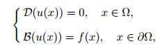
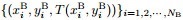
For a differential equation,
|
(3) |
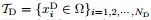
the input data are divided into boundary data 


|
(4) |
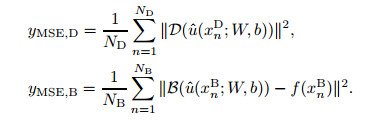
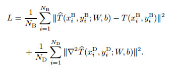
and the mean square errors are defined, respectively, as[14]
|
The optimization problem, which focuses on minimizing the loss function L with respect to W and b, consumes much more computing resources than the function approximator. Therefore, a second-order optimizer is used here. All the following examples in this section are optimized using the limited-memory Broyden-Fletcher-Goldfarb-Shanno (L-BFGS) method[25].
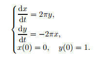
3.1 Ordinary differential equation (ODE) casesWe consider the following linear initial value problem:
|
(5) |
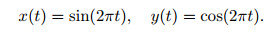
The ODE has solutions,
|
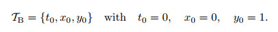
In the phase space, (x, y) is a unit circle, which is a visual indicator of the accuracy of the numerical solution. In this case, the boundary data are
|
The domain data are 

|
| Fig. 8 Solutions of the ODE system, where the small figure shows the orbit in the phase space (color online) |
|
|
A non-linear boundary value problem is also solved with the similar method. The second-order ODE defines a one-dimensional model of a boundary layer, where the parameter ν is the inverse of the Reynolds number,
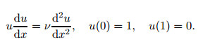
|
(6) |
With the special boundary condition, an explicit analytical solution does exist, i.e.,
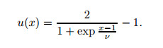
|
(7) |
The domain data are the same as those in the previous example, and the boundary data are 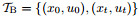
Figures 9 and 10 show the solutions and errors in two cases with different Reynolds numbers, demonstrating the high numerical accuracy of the NN solver for non-linear boundary value problems. The derivatives of the numerical solution obtained from the NN are calculated, and the calculated results are compared with the analytical solution. Similar to the interpolation capabilities of an NN, an NN solver contains information on the function to be solved as well as its derivatives, as shown in Figs. 11 and 12. Since Eq. (6) is a second-order ODE, there is no third- or fourth-order term in the training of Eq. (4), but the third-order derivative of the numerical solution in Fig. 13 is still consistent with the analytical result. The accuracy gets lower when it comes to the fourth order, as shown in Fig. 14, and the numerical solution has much stronger fluctuation than the analytical one.

|
| Fig. 9 The case of ν=0.007 with error distribution and average error, (a) comparison between numerical and exact solutions (color online), (b) point-wise absolute error of numerical solutions, where e=9.73×10⁻⁴ |
|
|

|
| Fig. 10 The case of ν=0.1 with error distribution and average error, (a) comparison between numerical and exact solutions (color online), (b) point-wise absolute error of numerical solutions, where e=8.28×10⁻⁵ |
|
|

|
| Fig. 11 First-order differentiation comparison, where e = 6.29 × 10⁻⁴ (color online) |
|
|

|
| Fig. 12 Second-order differentiation comparison, where e = 6.97 × 10⁻³ (color online) |
|
|

|
| Fig. 13 Third-order differentiation comparison, where e=5.55×10⁻² (color online) |
|
|

|
| Fig. 14 Fourth-order differentiation comparison, where e=2.19×10⁻¹ (color online) |
|
|
The Burgers equation and the heat equation are solved in this subsection. The Burgers equation is a one-dimensional simplified Navier-Stokes equation[14],
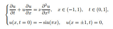
|
(8) |
where ν = 0.01/π is the reciprocal of the Reynolds number, similar to Eq. (6). The initial and boundary conditions are chosen such that a stable shock wave will propagate from the center of the spatial domain, which is a sensitive indicator of the numerical accuracy and stability of the algorithm. Solving Eq. (8) with the method described above[14] yields the result shown in Fig. 15.

|
| Fig. 15 Numerical solutions of the Burgers equation obtained with the NN (color online) |
|
|
The steady-state heat equation is

|
(9) |
This linear PDE can be solved analytically,
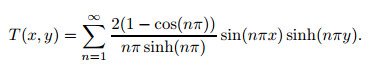
|
(10) |
The trial function 
|
Equation (9) is solved numerically by minimizing the loss function with respect to the weights and biases defined above. The L-BFGS second-order optimization method is used as a more efficient training method as it provides a higher convergence rate and lower gradient vanishing. Figure 16 shows the numerical and analytical results simultaneously. The analytical results are truncated at the first 40 terms for sufficient numerical accuracy. Figures 17-20 show that the solutions converge to a proper level as the number of collocation points in 


|
| Fig. 16 Contours in the heat equation, where the left and right parts are the numerical and analytical results, respectively (color online) |
|
|

|
| Fig. 17 NB=30, and ND=900 (color online) |
|
|

|
| Fig. 18 NB=60, and ND=3 600 (color online) |
|
|

|
| Fig. 19 NB=90, and ND=8 100 (color online) |
|
|

|
| Fig. 20 NB=120, and ND=14 400 (color online) |
|
|
We briefly describe NNs and the AD as a framework for solving ODEs and PDEs in this paper. We discuss our recent studies on the applications of NNs for use in the function approximation. We first show that using an NN as a fitting and interpolating tool for smooth, continuous but non-differentiable, and discontinuous functions yields results with high accuracy. Then, we use the method to numerically solve a series of differential equations, such as the one-dimensional boundary layer equation, the one-dimensional Burgers equation, and the two-dimensional steady-state heat equation.
We would like to point out that the ODE solver we develop is universal and produces results with the same level of accuracy as traditional numerical methods. There is no universal solver for PDEs, but some instances originating from physics and fluid dynamics are explored, and we obtain positive results. The main task for the current solver is to construct a valid loss function and to optimize it efficiently, for which the AD and L-BFGS methods can be efficient tools. An NN function approximator is also capable of providing differential information of the target function, rather than simply a set of discrete data points like the traditional numerical methods (e.g., the finite element method (FEM) and the finite volume method (FVM)). Moreover, working in complex geometries and dynamic resolution refinement are straightforward when using an NN function approximator.
Of course, there are obstacles that impede successful applications of NN methods. Processing the boundary conditions is challenging, i.e., some boundary conditions (e.g., boundary flux and non-slip boundary conditions) still impede the optimization convergence. Another problem is computational efficiency. NN methods usually consume much more computing resource than the finite difference method. However, new hardware (heterogeneous computing) and software (parallelization) can help overcome these challenges.
Our future work will focus on two main topics. First, we wish to enhance the accuracy of the results for examples where the convergence is guaranteed, especially PDEs. Second, we intend to develop a new way to construct a loss function such that the boundary condition becomes a constraint instead of a penalty, which will increase the accuracy of the numerical solution.
Aside from numerically solving PDEs, we believe that the use of NN for the function approximation could be used to analyze data from fluid experiments, especially the boundary layer data collected from hot-wire anemometer and particle image velocimetry (PIV) experiments[26-29]. Our idea is to feed the PIV experiment data into the NN model defined in Eq. (4) to obtain more accurate reconstruction of the fluid field.
| [1] |
VAN GERVEN, M. and BOHTE, S. Artificial neural networks as models of neural information processing. Frontiers in Computational Neuroscience, 11, 00114 (2017) doi:10.3389/fncom.2017.00114 |
| [2] |
HAYKIN, S. S. Neural Networks and Learning Machines, 3rd ed. Prentice Hall, Englewood, New Jersey (2008)
|
| [3] |
KRIZHEVSKY, A., SUTSKEVER, I., and HINTON, G. E. Imagenet classification with deep convolutional neural networks. Proceedings of the 25th International Conference on Neural Information Processing Systems, 1, 1097-1105 (2012) |
| [4] |
LECUN, Y., BENGIO, Y., and HINTON, G. Deep learning. nature, 521, 436-444 (2015) doi:10.1038/nature14539 |
| [5] |
LAKE, B. M., SALAKHUTDINOV, R., and TENENBAUM, J. B. Human-level concept learning through probabilistic program induction. Science, 350, 1332-1338 (2015) doi:10.1126/science.aab3050 |
| [6] |
ALIPANAHI, B., DELONG, A., WEIRAUCH, M. T., and FREY, B. J. Predicting the sequence specificities of DNA-and RNA-binding proteins by deep learning. Nature Biotechnology, 33, 831-838 (2015) doi:10.1038/nbt.3300 |
| [7] |
MCCULLOCH, W. S. and PITTS, W. A logical calculus of the ideas immanent in nervous activity. The Bulletin of Mathematical Biophysics, 5, 115-133 (1943) doi:10.1007/BF02478259 |
| [8] |
ROSENBLATT, F. The perceptron:a probabilistic model for information storage and organization in the brain. Psychological Review, 65, 386-408 (1958) doi:10.1037/h0042519 |
| [9] |
ROSENBLATT, F. Principles of Neurodynamics:Perceptions and the Theory of Brain Mechanism, Spartan Books, Washington, D. C (1961)
|
| [10] |
MINSKY, M. and PAPERT, S. A. Perceptrons:An Introduction to Computational Geometry, MIT Press, Cambridge (1969)
|
| [11] |
WERBOS, P. Beyond Regression: New Tools for Prediction and Analysis in the Behavioral Sciences, Ph. D. dissertation, Harvard University (1974)
|
| [12] |
RALL, L. B. Automatic Differentiation:Techniques and Applications, Springer-Verlag, Berlin (1981)
|
| [13] |
BAYDIN, A. G., PEARLMUTTER, B. A., RADUL, A. A., and SISKIND, J. M. Automatic differentiation in machine learning:a survey. The Journal of Machine Learning Research, 18, 1-43 (2018) |
| [14] |
RAISSI, M., PERDIKARIS, P., and KARNIADAKIS, G. E. Physics informed deep learning (part i): data-driven solutions of nonlinear partial differential equations. arXiv, arXiv: 1711.10561(2017) https://arxiv.org/abs/1711.10561
|
| [15] |
MALL, S. and CHAKRAVERTY, S. Application of legendre neural network for solving ordinary differential equations. Applied Soft Computing, 43, 347-356 (2016) doi:10.1016/j.asoc.2015.10.069 |
| [16] |
MALL, S. and CHAKRAVERTY, S. Chebyshev neural network based model for solving laneemden type equations. Applied Mathematics and Computation, 247, 100-114 (2014) doi:10.1016/j.amc.2014.08.085 |
| [17] |
BERG, J. and NYSTRÖM, K. A unified deep artificial neural network approach to partial differential equations in complex geometries. arXiv, arXiv: 1711.06464(2017) https://arxiv.org/abs/1711.06464
|
| [18] |
MAI-DUY, N. and TRAN-CONG, T. Numerical solution of differential equations using multiquadric radial basis function networks. Neural Networks, 14, 185-199 (2001) doi:10.1016/S0893-6080(00)00095-2 |
| [19] |
JIANYU, L., SIWEI, L., YINGJIAN, Q., and YAPING, H. Numerical solution of elliptic partial differential equation using radial basis function neural networks. Neural Networks, 16, 729-734 (2003) doi:10.1016/S0893-6080(03)00083-2 |
| [20] |
ABADI, M., BARHAM, P., CHEN, J., CHEN, Z., DAVIS, A., DEAN, J., DEVIN, M., GHEMAWAT, S., IRVING, G., ISARD, M., and KUDLUR, M. Tensorflow:a system for large-scale machine learning. The 12th USENIX Symposium on Operating Systems Design and Implementation, 16, 265-283 (2016) |
| [21] |
HORNIK, K., STINCHCOMBE, M., and WHITE, H. Multilayer feedforward networks are universal approximators. Neural Networks, 2, 359-366 (1989) doi:10.1016/0893-6080(89)90020-8 |
| [22] |
CYBENKO, G. Approximation by superpositions of a sigmoidal function. Mathematics of Control, Signals and Systems, 2, 303-314 (1989) doi:10.1007/BF02551274 |
| [23] |
JONES, L. K. Constructive approximations for neural networks by sigmoidal functions. Proceedings of the IEEE, 78, 1586-1589 (1990) doi:10.1109/5.58342 |
| [24] |
CARROLL, S. and DICKINSON, B. Construction of neural networks using the Radon transform. IEEE International Conference on Neural Networks, 1, 607-611 (1989) |
| [25] |
LIU, D. C. and NOCEDAL, J. On the limited memory BFGS method for large scale optimization. Mathematical Programming, 45, 503-528 (1989) doi:10.1007/BF01589116 |
| [26] |
LEE, C. B. Possible universal transitional scenario in a flat plate boundary layer:measurement and visualization. Physical Review E, 62, 3659-3670 (2000) doi:10.1103/PhysRevE.62.3659 |
| [27] |
LEE, C. B. and WU, J. Z. Transition in wall-bounded flows. Applied Mechanics Reviews, 61, 030802 (2008) doi:10.1115/1.2909605 |
| [28] |
LEE, C. B. New features of CS solitons and the formation of vortices. Physics Letters A, 247, 397-402 (1998) doi:10.1016/S0375-9601(98)00582-9 |
| [29] |
LEE, C. B. and FU, S. On the formation of the chain of ring-like vortices in a transitional boundary layer. Experiments in Fluids, 30, 354-357 (2001) doi:10.1007/s003480000200 |