
 2019, Vol. 40
Shanghai University
Article Information
- TAN Ying, SU Weidong
- A trigonometric series expansion method for the Orr-Sommerfeld equation
- Applied Mathematics and Mechanics (English Edition), 2019, 40(6): 877-888.
- http://dx.doi.org/10.1007/s10483-019-2484-9
Article History
- Received Mar. 7, 2018
- Revised Nov. 25, 2018


2. Department of Mechanics and Engineering Science, College of Engineering, Peking University, Beijing 100871, China
The study of the linear stability of viscous parallel flows, e.g., plane Poiseuille flow (PPF), plane Couette flow (PCF), and boundary layer flow, plays a key role in predicting transition by means of semi-empirical methods, such as eN for a more precise evaluation for the performances of many industrial apparatuses that involve fluids. These flows occur in various slit flows with rest and moving units, micro-flows in channels, and flows near the surfaces of aircrafts and blades of fluid machineries. The governing equation describing the linear disturbances in viscous parallel flows is the classical Orr-Sommerfeld equation, which is a fourth-order linear ordinary differential equation involving the known base flow. While analytical solutions are very difficult to obtain or hard to work with, mature numerical methods for solving the Orr-Sommerfeld equation have been developed for a long time. Thomas[1] for the first time solved the equation of PPF using the finite difference method on a computer and found a critical Reynolds number of 5 780. Subsequently, there has been a series of spectral methods relying on special orthogonal basis function expansion such as those suggested by Dolph and Lewis[2], Gallagher and Mercer[3], and Grosch and Salwen[4]. The method based on Chebyshev polynomials expansion was developed by Orszag[5], and the results have been used as the benchmark extensively over the years. Herbert[6] applied the Chebyshev spectral method, requiring the control equations to be satisfied exactly at the collocation points, to the Orr-Sommerfeld equation. In recent years, this method has turned out to be more attractive to many researchers in solving a variety of stability problems, since the computation is accurate and efficient. However, the Chebyshev spectral collocation method is much dependent on the selection of collection points, and at the same time, when the number of modes increases, the computation gives rise to a certain degree of instability.
It is well known that trigonometric functions are the most convenient orthogonal basis functions applicable to the spectral methods for solving differential equations. However, it is surprising that this elementary method has never appeared in the literature pertaining to numerically solving the Orr-Sommerfeld equation (it was mentioned by Zhou et al.[7] that trigonometric functions were used earliest as basis functions to solve the Orr-Sommerfeld equation but the result was not ideal). Hence, in this paper, we develop such a method and two similar modified ones for the Orr-Sommerfeld equation. The method is based on a trigonometric series expansion with an auxiliary function and then uses the weighted residual method and Lanczos's tau method[8], which provides an alternative to the current Chebyshev spectral methods and may be applied to the study of linear stability problems. It produces the matrices of the moderate size, which provide an approximation of the set of eigenvalues and corresponding eigenfunctions. At the same time, our method is easier to implement than other usual methods and yields accurate results. Moreover, compared with the finite difference method, it requires fewer modal numbers and fewer computer time, and compared with the Chebyshev collocation method, when the modal number increases, our method is better in the performance of stability.
In Section 2, the formulation and implementation procedure of the method are presented. Then, in Section 3, we apply the method to five test cases. In the first two cases, we calculate two canonical flows, the PPF and the PCF. In the third case, to illustrate the wide applicability of our method, we investigate the influence of the Navier slip boundary on the stability of the PPF. It is well known that, in many fluid regimes, for instance, the micro-channel flow[9] and the moving contact line problem[10], the slip boundary may play a significant role. In the fourth case, we choose to study the influence of a new form of boundary condition on the stability of the PCF, in order to further show the advantages of our method. In the last case, we investigate the Blasius boundary layer and obtain satisfactory results. Finally, the conclusions are summarized in Section 4.
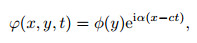
2 Trigonometric series expansion method for the Orr-Sommerfeld equation 2.1 Orr-Sommerfeld equation for plane parallel flowsFor the linear stability analysis of an incompressible viscous flow with a single streamwise velocity in the region -1≤ y≤ 1 bounded by two parallel infinite walls, the stream function for a two-dimensional disturbance is assumed to be of the form
|
(1) |
where α and c denote the real disturbance wavenumber and complex wave speed, respectively. Here, we consider the temporal stability problem.
Introducing the above representation into the linear partial differential equation satisfied by the disturbance stream function φ(x, y, t), we obtain the following Orr-Sommerfeld equation:

|
(2a) |
with the conventional boundary conditions

|
(2b) |
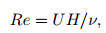
where D=d/dy, U(y) is the real mean streamwise velocity, and Re is the Reynolds number defined as
|
in which U is the characteristic velocity, H is the real distance between the two walls at rest, and ν is the kinematic viscosity. All the quantities and the coordinates in Eqs. (1) and (2) are non-dimensional. For any given Re and α, Eq. (2) constitutes an eigenvalue problem with c to be solved.
In Eq. (1), if αc is set to be a known real number while regarding α as an unknown complex number, the problem is called the spatial stability problem. This leads to a nonlinear (polynomial) or algebraic eigenvalue problem which is more difficult to tackle, since α2, α3, and α4 are involved in the Orr-Sommerfeld equation. Moreover, the temporal stability problem is more elementary in many cases. Therefore, only temporal stability is analyzed in the present study.
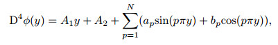
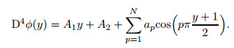
2.2 A trigonometric series expansion methodThis method, which is called a trigonometric series expansion method, is developed as a spectral method to solve the eigenvalue problem formulated by Eq. (2). The specific procedure is presented as follows. In terms of the idea of trigonometric series expansion, we expand the highest derivative of ϕ in Eq. (2) into the trigonometric series with a linear function appended, i.e.,
|
(3) |
where ap and bp are the expansion coefficients with A1 and A2 being the constants. Here, since we are not sure whether the highest order derivative in the governing equation, i.e., D4ϕ, can be periodically continued without jumping points, a linear auxiliary function A1y+A2 as the simplest form is introduced to separate the non-periodic component of the fourth derivative function. This technique serves to improve the accuracy of the approximation, and shall be further presented in the end of the section.
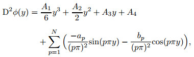
Starting from the series representation of the fourth-order derivative, all of the lower order derivatives of the eigenfunctions can be obtained by integrating the expansion (3) successively as

|
(4a) |
|
(4b) |
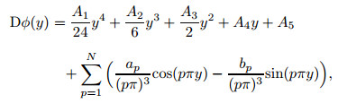
|
(4c) |
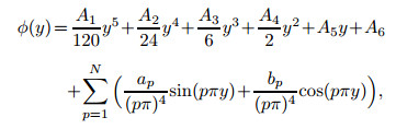
|
(4d) |
where A3, A4, A5, and A6 are the constants of integration, and here we put them all as coefficients to be determined. In other words, they have the same status as ap and bp.
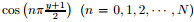
Next, we substitute Eq. (4) into Eq. (2a), and use the usual weighted residual method procedure, herein sin(nπy) and cos(nπy)(n=0, 1, 2, ..., N) are used as the weight functions. A generalized matrix eigenvalue problem of the form
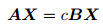
|
(5) |
can be obtained finally, where A and B are the coefficient matrices containing Re and α, and X is a column vector of the form

|
(6) |
The boundary conditions are dealt with using the idea of Lanczos's tau method[6]. Specifically, substituting Eq. (4) into Eq. (2b) for the discretized boundary conditions, we get another four equations. In other words, there are 2(N+1) equations from the governing equation (2a) and four equations from the boundary conditions (2b) in all of the 2N+6 unknowns. At this point, we get a well-posed problem and then the eigenvalue c can be evaluated numerically, say, by the MATLAB® function eig(B-1A) as used in this paper.
Furthermore, according to the idea that a function can be extended by odd prolongation or even prolongation, we can also expand the highest order derivative of ϕ in Eq. (2) into a truncated sine or cosine series as follows:
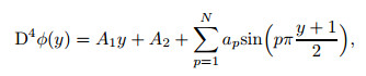
|
(7) |
or
|
(8) |
Here, we call them a modified sine or cosine series expansion method. The specific procedures are similar to the preceding trigonometric series expansion method and hence the relevant details are not presented any longer. In particular, 
The convergence rate of these methods can be easily known through the property of trigonometric series expansions. For the fourth-order derivative function, the series approximate only a continuous periodic function without jumping points. The nth expansion coefficient tends to zero at a rate of n-2 at least, and this corresponds to a convergence rate of first order at least for the truncated series. By successive integrations, the performance of convergence is progressively improved. The final convergence rate for the stream function itself will be fourth order at least. This accuracy of approximation is enough for most problems.
It should be emphasized that our approach belongs to the Galerkin spectral method. Therefore, no discrete grids or collocation points are needed. The only input parameter is the number of truncated modes in the trigonometric series expansions. Moreover, these methods can also be applied with no difficulty to the Orr-Sommerfeld equation with other possible homogeneous boundary conditions. The validation of the methods will be shown below.
3 Test casesIn this section, the trigonometric series expansion method and two modified methods are applied to solve the Orr-Sommerfeld equation in linear stability problems of plane parallel shear flows under both the standard equation (2b) and distinctive homogeneous boundary conditions.
3.1 PPFHere, the basic flow velocity in the x-direction is
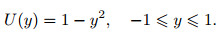
|
(9) |
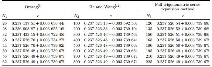
For this problem, the results of Orszag[5] obtained by the Chebyshev polynomials method are benchmark, and the finite difference method used by He and Wang[11], which was developed by Thomas[1], is also one of the conventional methods.
In Table 1, we show the convergent results of the most unstable eigenvalue c computed by our trigonometric series expansion method with the disturbance wavenumber α =1 and the Reynolds number Re=10 000, along with the comparison to those results obtained by Orszag[5] and He and Wang[11]. Here, N3 is the number of terms of truncated trigonometric series expansion, N2 is the number of grid points of the finite difference method, and N1 is the number of terms of the truncated Chebyshev polynomials. The eigenvalue generated by our method with N3=165 or so, is found to converge to 0.237 526 50+0.003 739 67i, which agrees with the precise result to 8 significant digits. In addition, it is well known that the unstable eigenmode of PPF is symmetric. Therefore, we can take simpler expansion for the highest derivative of ϕ as

|
(10) |
to further reduce the cost of calculation. It is shown in Table 1 that our method uses much fewer truncated modes than the number of grid points in the finite difference method using uniform grid points. This means the lesser computation scale since the formed matrices A and B have lesser order. It is known that certain optimally selected non-uniform grid in the finite difference method can drop the number of grid to some degree. However, we have found that the cost of computation under such strategy is still much higher than the suggested trigonometric function method as further demonstrated below.
The eigenvalues for the first 10 most unstable modes obtained by our trigonometric series expansion method and Orszag[5] are compared in Table 2. Accurate to eight decimal digits, the results are exactly the same.

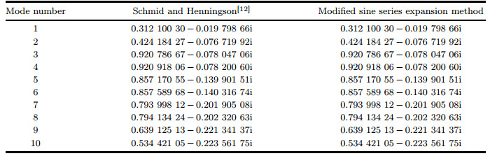
For the same disturbance wavenumber but Reynolds number Re=2 000, using our modified sine series expansion method, the first 10 most unstable eigenvalues are obtained and compared with the results obtained by means of the Chebyshev collocation method by Schmid and Henningson[12], as listed in Table 3.
The neutral curve for the PPF is shown in Fig. 1, together with contours of the constant nonzero growth rate ci. At the same time, we find that the critical Reynolds number Re=5 772.22 with the wavenumber αc=1.020 56 is consistent with the previous results.

|
| Fig. 1 Neutral stability curve and contours of the constant growth rate for the PPF by the modified sine series expansion method |
|
|
With regard to the computation cost, it is worth pointing out that, although our methods using the trigonometric series expansion require more modes than the Chebyshev collocation method, we find that the computing time is basically on the same order as the latter for the Reynolds number of 2 000 and α=1. Specifically, the computation time for the Chebyshev collocation method and that for the trigonometrical method are about 0.08 s and 0.22 s on our computer, respectively. The main computational complexity comes from the order of the coefficient matrix A or B. Our calculations indicate that the modal number of the trigonometrical functions expansion method is higher than that of the Chebyshev collocation method when obtaining the eigenvalue with the same accuracy. Thus, the computation cost for the former is higher than that for the latter. With an accuracy of 8 digits for the most unstable eigenvalue at the Reynolds number of 10 000 and α=1, we find that the computing time of the former and the latter is about 0.12 s and 0.80 s on our computer, respectively. The computation time under the same parameters for the finite difference method used by He and Wang[11] is not available to us. However, the computational complexity with N3=225 for the trigonometrical functions expansion should be comparable with N2=800 for the finite difference method. It should be emphasized that the main advantage of our approach is not only the computational efficiency but also the robustness when increasing the truncated modal number, as shown in the other cases presented below.
3.2 PCFThe corresponding basic flow velocity to the PCF in the x-direction is
|
(11) |
In Table 4, the first 10 most unstable eigenvalues for α =1 and Re=800 are listed, which are computed by our trigonometric series expansion method and the Chebyshev collection method in Ref. [12], respectively. It is clear that they both converge to the same values, except for some minute difference after the 8th significant digits for some modes. Figure 2 shows the contours of the growth rate for the PCF. It is well known that the spectra of PCF do not contain any unstable eigenvalues for any parameter combinations.


|
| Fig. 2 Contours of the constant growth rate for the PCF by the modified sine series expansion method |
|
|
Here, we consider the PPF with the Navier slip boundary conditions[11]

|
(12) |
at the wall, where ls is the slip length, and n is the normal unit vector pointing to the interior of the fluid. For the stream function of the two-dimensional disturbance, the boundary conditions read
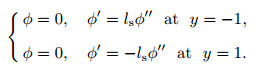
|
(13) |
The mean velocity for this problem is given by
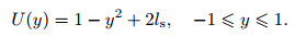
|
(14) |
Obviously, ls=0 corresponds to the no-slip boundary condition. We consider the case with α =1, Re=100 000, and ls=0.008.
The most unstable eigenvalue c computed by our trigonometric series expansion method is listed in Table 5. Comparing the results with those of He and Wang[11] obtained by the Chebyshev collocation method and the finite difference method, it is found that the eigenvalue converges to the same value 0.243 260 44 + 0.002 270 66i.
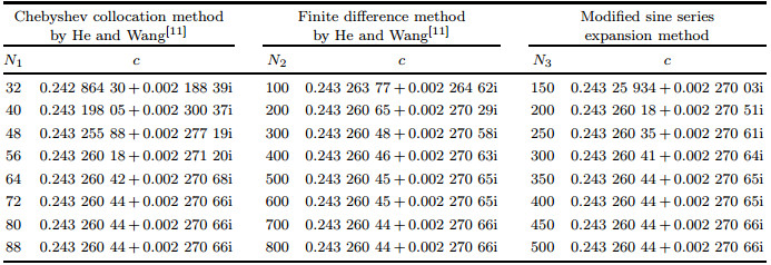
Figure 3 shows the neutral curves of the PPFs with slip boundaries of ls=0, 0.004, and 0.008, respectively. It is clear that the critical Reynolds number increases as the slip length increases. In other words, the Navier slip of the wall increases the stability of the flow. Our conclusion is in conformity with that of He and Wang[11].

|
| Fig. 3 Neutral stability curves for the PPF with different slip lengths by the modified sine series expansion method |
|
|
The channel flow with a slip boundary is frequently introduced as an appropriate model in micro-fludics, which is related to enormous applications in biomedical, chemical, and mechanical engineering. More potential applications for flows with slip boundaries may be expected in the future. Hence, the study on the corresponding hydrodynamical instability becomes more and more important.
3.4 PCF under a new form of boundary conditionsHere, we first propose a new form of boundary conditions

|
(15) |
For the PCF, the new boundary conditions can be expressed in terms of the stream function,

|
(16) |
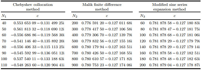
Now, we still consider the basic flow with the form of Eq. (11). Only the boundary conditions for the disturbance velocity are new. Since the problem has never been calculated, we use three different methods to solve this new problem in order to obtain the credible result. For α =1 and Re=800, the eigenvalues are obtained by our modified sine series expansion method and listed in Table 6. Meanwhile, the results calculated by the Chebyshev collection method and the compact finite difference method[13] are also presented for comparison.
|
It is shown that our method and the finite difference method produce basically the same results. Compared with the accuracy of 5 decimal digits obtained by our method, the Malik compact finite difference method could only guarantee the accuracy of 2 decimal digits. Unfortunately, we cannot get credible eigenvalues by the Chebyshev collocation method this time, since the results do not converge as the number of truncated modes increases. Here, we choose the Gauss-Lobatto collocation points, and we do not rule out the possibility that using other forms of collocation points may improve this situation.
3.5 Blasius boundary layer flowThe most remarkable difference among the Blasius boundary layer flow, the PPF Poiseuille flow, and the PCF is that the boundary of the first one is a semi-infinite region, while the latter two are finite regions. Under the approximately parallel hypothesis, the corresponding basic flow velocity to the Blasius boundary layer flow is directly given by the well-known Blasius equation. Here, the velocity profile is obtained by numerical integration.
Note that the displacement thickness is used as the characteristic length. For α =0.308 and Re=998, the convergent results of the most unstable eigenvalue are shown in Table 7. It is observed that as the number of collocation points N1 increases, the result quickly converges, but with N1 continuing to grow, the result begins to sparse. When the number of truncation terms for the trigonometric series N3 is around 130, the results given by the modified sine series expansion method converge to 0.364 2 + 0.007 9i, which agree well with the result calculated by Antar[14]. Meanwhile, the result is very stable as N3 continues to grow. The computed critical Reynolds number is around 520, which is consistent with the numerical result by Jondinson[15]. Moreover, we find that whereas the Chebyshev collocation method is significantly dependent on the selection of the number of the collocation points in the calculation of eigenvalues of the flow, the trigonometric series expansion method is weakly dependent on the number of truncated terms when the number is large enough. For the need of using a variety of convenient methods to arrive at the credible results in the calculation of similar problems, here we come up a simple and even more robust alternative to the present popular methods as shown in the above analysis.

|
In this work, we develop an integral trigonometric series expansion method with auxiliary functions and two similar modified methods for solving the Orr-Sommerfeld equation. To verify our approach, we perform five numerical cases, the PPF with both no-slip and slip boundary conditions, the PCF with no-slip as well as a new form of boundary conditions, and the Blasius boundary layer with the no-slip boundary condition, respectively. As a kind of spectral methods, we show that these proposed methods possess comparatively much rapid convergence compared with the finite difference method and better robustness compared with the Chebyshev collocation method. Since the elementary basis functions are adopted, this approach is much easier to implement than the conventional spectral methods that use more complicated basis functions. In particular, because of their robustness, when increasing the modal number, the present methods can also serve as suitable alternatives in finding reliable eigenvalues when dealing with hydrodynamic stability problems.
Our approach can be readily extended to the three-dimensional disturbance problem. Moreover, it can be readily used to tackle more stability problems with boundary conditions of general types, such as the Navier slip boundary conditions and the other one mentioned above. Moreover, it can be applied to investigate those problems which can be simplified as homogeneous or non-homogeneous higher order linear ordinary differential equations similar to the Orr-Sommerfeld equation, such as the stability of parallel viscous mixing layers with two phases, elastic stability, and combustion stability. Overall, it can be expected that the presented trigonometric series methods will be effective as well for dealing with more boundary-value or eigenvalue problems of linear ordinary differential equations.
Acknowledgements The authors would like to thank the reviewers for valuable comments. We also thank Dr. Yuning HUANG for helpful suggestions on the manuscript.
| [1] |
THOMAS, L. H. The stability of plane Poiseuille flow. Physical Review, 91(4), 780-783 (1953) doi:10.1103/PhysRev.91.780 |
| [2] |
DOLPH, C. L. and LEWIS, D. C. On the application of infinite systems of ordinary differential equations to perturbations of plane Poiseuille flow. Quarterly of Applied Mathematics, 16(2), 97-110 (1958) doi:10.1090/qam/1958-16-02 |
| [3] |
GALLAGHER, A. P. and MERCER, A. M. On the behaviour of small disturbances in plane Couette flow. Journal of Fluid Mechanics, 13(1), 91-100 (1962) |
| [4] |
GROSCH, C. E. and SALWEN, H. The stability of steady and time-dependent plane Poiseuille flow. Journal of Fluid Mechanics, 34(1), 177-205 (1968) doi:10.1017/S0022112068001837 |
| [5] |
ORSZAG, S. A. Accurate solution of the Orr-Sommerfeld stability equation. Journal of Fluid Mechanics, 50(4), 689-703 (1971) doi:10.1017/S0022112071002842 |
| [6] |
HERBERT, T. Analysis of the subharmonic route to transition in boundary layers. 22nd Aerospace Sciences Meeting, American Institute of Aeronautics and Astronautics, New York (1984) http://adsabs.harvard.edu/abs/1984aiaa.meetV....H
|
| [7] |
ZHOU, H. and ZHAO, G. F. Hydrodynamic Stability (in Chinese), National Defence Industrial Press, Beijing (2004)
|
| [8] |
LANCZOS, C. Applied Analysis, Prentice Hall, Englewood Cliffs (1956)
|
| [9] |
GAD-EL-HAK, M. The fluid mechanics of microdevices-the freeman scholar lecture. Journal of Fluids Engineering, 121(1), 5-33 (1999) doi:10.1115/1.2822013 |
| [10] |
QIAN, T., WANG, X. P., and SHENG, P. A variational approach to the moving contact line hydrodynamics. Journal of Fluid Mechanics, 564, 333-360 (2006) doi:10.1017/S0022112006001935 |
| [11] |
HE, Q. and WANG, X. P. The effect of the boundary slip on the stability of shear flow. Zeitschrift für Angewandte Mathematik und Mechanik, 88(9), 729-734 (2008) doi:10.1002/zamm.v88:9 |
| [12] |
SCHMID, P. J. and HENNINGSON, D. S. Stability and Transition in Shear Flows, Springer, New York (2001) https://www.springer.com/us/book/9780387989853
|
| [13] |
MALIK, M. R. Numerical method for hypersonic boundary layer stability. Journal of Computational Physics, 86, 376-413 (1990) doi:10.1016/0021-9991(90)90106-B |
| [14] |
ANTAR, B. N. The eigenvalue spectrum of the Orr-Sommerfeld problem. NASA STI/Recon Technical Report N, 77N11344, NASA, Washington, D. C. (1976) https://www.researchgate.net/publication/24330935_The_eigenvalue_spectrum_of_the_Orr-Sommerfeld_problem
|
| [15] |
JONDINSON, R. The flat plate boundary layer, part 1, numerical integration of the OrrSommerfeld equation. Journal of Fluid Mechanics, 43(4), 801-811 (1970) doi:10.1017/S0022112070002756 |