1 Introduction

Let Ω be a bounded, connected, Lipschitz continuous domain of , and Γ be the boundary of Ω. We consider the incompressible convective Brinkman-Forchheimer equations,

(1)

(2)

(3)

where u=(u₁, u₂)=(u₁(x), u₂(x)) represents the velocity vector, p=p(x) denotes the pressure, f=(f₁(x), f₂(x)) represents the prescribed body force, and ν>0 is the Brinkman coefficient (or the effective viscosity). Let |·| denote the Euclidean norm, and . The Forchheimer term α|u|^r-2u with coefficients α>0 and 2≤ r < ∞ is derived from Forchheimer's law^[1], which describes various physical situations, such as a porous media flow, drag, or friction effects, as well as certain dissipative mechanisms^[1-7]. There are three widely used forms corresponding to different values of α and r in the Forchheimer term, that is, the Darcy term αu for r=2, the Forchheimer term α|u|u for r=3, and the Forchheimer term α|u|²u for r=4. Therefore, α denotes the Darcy or Forchheimer coefficient. From a mathematical viewpoint, the incompressible Brinkman-Forchheimer equations are a nonlinear reaction-convection-diffusion problem, which exhibits a convection-dominated or reaction-dominated property for a small Brinkman coefficient ν.

A theoretical analysis of partial differential equations (PDEs) with the term |u|^r-2u (r≥2), called the damping term or source term in the references, has been extensively investigated during the last few decades. For example, in Refs. [3], [4], and [8], the authors pointed out that the source term |u|^r-2u can lead to a finite time blow-up of a solution to linear hyperbolic problems. In Ref. [9], a detailed analysis of the systems of hyperbolic conservation laws with damping and relaxation was proved. In Ref. [2], the zero viscosity limit of lengthy averages of the solutions to the Navier-Stokes equations with the linear damping term γu was established. In Refs. [10] and [11], global attractors of Navier-Stokes equations or g-Navier-Stokes equations with the linear damping term αu were investigated.

It is well known that a Darcy flow describes the creeping flow of Newtonian fluids in porous media. However, Forchheimer^[1] found the relationship between the pressure gradient and the Darcy velocity to be nonlinear for moderate Reynolds numbers. He observed that the nonlinear term appears to be quadratic, and formulated the Darcy-Forchheimer equations^{[1, 6]}. In these cases, the nonlinear inertial term becomes insignificant. The Brinkman-Forchheimer equations can be considered as an extension of the Darcy-Forchheimer equations when the inertial effects cannot be neglected^[12-14], which has been used to describe the motion of an incompressible fluid flow in saturated porous media^[15-16] or a non-Newtonian fluid^[17]. Incompressible convective Brinkman-Forchheimer equations can be obtained in different ways. In Ref. [12], the local volume averaging technique was used to establish the governing equations, and in Ref. [13], the nonlinear Forchheimer drag law, rather than the linearized (Darcy) drag law, was used to derive the governing equations.

Recently, some asymptotic behaviors and continuous properties of the solutions to Brinkman-Forchheimer equations have been studied in Refs. [5] and [18]-[20] and the references therein. In Ref. [5], the approximation of the solutions to the three-dimensional convective Brinkman-Forchheimer equations was discussed. The existence of a global attractor for the Brinkman-Forchheimer equations in the phase space H₀¹(Ω) was studied^[18-19]. In Ref. [20], the existence of regular dissipative solutions and global attractors for the three-dimensional Brinkmann-Forchheimer equations with a nonlinearity of an arbitrary polynomial growth rate was derived. In Ref. [21], the continuous dependence of the solutions to the unsteady Brinkman-Forchheimer equations on the Brinkman and Forchheimer coefficients in an H¹ norm was proved. In Ref. [22], the convergence and continuous dependence for the Brinkman-Forchheimer equations with the temperature field were presented.

Problems (1)-(3) are nonlinear and of a monotone type owned by the Forchheimer term α|u|^r-2 u. Recently, a numerical analysis of problems (1)-(3) without the convection term (u·▽)u was presented^[23-24], which showed that the flow is a creeping flow. In Ref. [23], the existence and uniqueness of the weak and discrete solutions were proved, and the error estimates of the conforming finite element approximation and numerical result were presented. In Ref. [24], the superconvergence properties of the conforming mixed finite element methods were considered.

The purpose of this paper is to consider the numerical analysis for the incompressible convective Brinkman-Forchheimer equations. Owing to the arrival of the Forchheimer term α|u|^r-2 u (r≥ 2), further analysis is required to establish the corresponding theory. In this paper, we focus on a conforming finite-element approximation for problems (1)-(3), and establish the existence, uniqueness, and error estimation of the continuity and approximation problem. In addition, some numerical schemes are presented and tested.

The remainder of this paper is organized as follows. In Section 2, we provide some facts regarding the Sobolev spaces and introduce the variational problem of incompressible Brinkmann-Forchheimer equations (1)-(3). In Section 3, based on the Galerkin method and a saddle-point argument, we establish the existence, uniqueness, and stability of a weak solution to the variational problem, and establish the convergence of a weak solution to the Brinkman-Forchheimer equations to a weak solution to the Navier-Stokes equation as the Forchheimer coefficient α tends toward zero. In Section 4, we establish the existence and uniqueness of the conforming finite element approximation. The remaining part of this section focuses on establishing the error estimates. In Section 5, we study some numerical schemes, and propose the one-step Newton (or semi-Newton) iteration method initialized using a fixed-point iteration. In Section 6, a numerical experiment conducted using a Taylor-Hood finite element is described. We test several examples using structured and unstructured triangular meshes for different selections of the Brinkman coefficient ν, the Forchheimer coefficient α, and the parameter r. Finally, some concluding remarks are provided in Section 7.

2 Functional setting and variational problem

For the mathematical setting of problems (1)-(3), we introduce the Sobolev spaces X and M, i.e.,

The space X is separable and equipped with the norm^[25],

According to the Sobolev imbedding theorem^[26], we have , and for a positive constant c₁. Thus, for r ∈[2, ∞), the space X=H₀¹(Ω), and the norm ‖·‖_{1, 2} is the equivalent norm of space X, that is, there exist two positive constants c₂ and c₃ such that ∀u ∈ X,

is satisfied. The space M is equipped with the usual L² norm. Next, let the closed subset V of X be given by

In addition, c or c_i (i=1, 2, ...) denotes a general positive constant.

We introduce the following bilinear, trilinear, and quasi-bilinear forms:

It is well known that^{[10, 23, 26-27]}

(4)

(5)

(6)

(7)

(8)

(9)

(10)

where

is a definite number, and is the conjugate number of r.

Using (4), (5), (9), and (10), we have the following lemmas.

Lemma 1   The quasi-bilinear form a(·;·, ·) is coercive on X, i.e.,

Lemma 2    The mapping u→ a(u; u, v) is sequentially weakly continuous on X, i.e., if in X, then

Proof   Note that

(11)

Clearly, I₁→ 0 as m→∞. In contrast, using the following inequality^[29]:

(12)

∀u, v, w ∈ X, we obtain

Hence,

(13)

Moreover, , and ‖u_m‖_{0, r} and ‖u‖_{0, r} are bounded. Meanwhile, ‖u_m-u‖_{0, r}→ 0 as m→∞. Combining the above conclusions yields the result.

With the above notations, the variational formulation of problems (1)-(3), called Problem (Q), reads as follows. For the given f ∈ X', find (u, p)∈ X× M such that for all (v, q)∈ X× M,

(14)

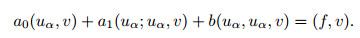
Associated with Problem (Q), we introduce the following equivalence problem, called Problem (P). For the given f ∈ V', find u ∈ V such that for all v ∈ V,

(15)

3 Existence and uniqueness of variational problem

In this section, we study the existence and uniqueness of the variational problems (Q) and (P), and present an a priori estimate of the solution to the variational problem. First, we establish the following existence and uniqueness theorem for Problem (P).

Theorem 1   Let Ω be a bounded set in , and f be given in V'. Thus, there exists at least one solution u ∈ V, which satisfies the following priori estimate:

(16)

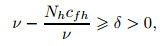
such that Problem (P) is satisfied. Moreover, if ν is sufficiently large or f is sufficiently small such that

(17)

then there exists a unique solution to Problem (P). In the above, the constant

Proof   First, the existence of the solution to Problem (P) is proved using the Galerkin method. Noting that the space V is a subspace of X, there exists a sequence w_i (i=1, 2, ...) of linearly independent elements of V. For each fixed integer m≥0, we denote the finite dimensional subspace V_m= span{w_i}_i=1^m⊂ V, and define the Galerkin approximation solution u_m ∈ V_m of Problem (P) as

(18)

(19)

(18) and (19) make up a nonlinear system of the coefficients ξ_{i, m} (i=1, 2, ..., m). To prove the solvability of the system, we introduce the operator S_m, i.e.,

Clearly, S_m is continuous. Moreover, by using the inequalities (5) and (10), as well as Lemma 1, we obtain ∀u, v ∈ V_m,

(20)

Note that the quantity ‖·‖_{1, 2} is the equivalent norm of the space X. It follows that 〈 S_m(u), u 〉 >0 for . Using the fixed point lemma in Refs. [27] and [28], there exists a solution u_m to Problem (P) in the closed sphere B(k)={u ∈ X, ‖u‖_X≤ k}.

We multiply ξ_{k, m} on both sides of (19), and sum the equalities for k=1, 2, ..., m. Then, we obtain

(21)

Because of Lemma 1,

(22)

We deduce a priori estimate of ‖u_m‖ in V,

(23)

Hence, there exists u ∈ V and a weakly convergent subsequence, which is still denoted as u_m, such that

(24)

In contrast, the space X is compact when embedded into the space L²(Ω), and thus we obtain

(25)

Moreover, using Lemma 2, u is the solution to Problem (P).

Next, the uniqueness of Problem (P) is proved through a contradiction. Let u₁ and u₂ be two solutions to Problem (P), and denote u=u₁-u₂. We then have

(26)

Taking v=u in (26), and using the inequality^[30]

(27)

and the relations (4)-(10), we obtain

Now, from the condition (17), we have

which means that u₁=u₂, and the solution to Problem (P) is unique.

To study the existence and uniqueness of Problem (Q), we introduce the following "LBB" condition^[31].

Lemma 3    Let Ω be a bounded, connected, and Lipschitz continuous domain of , and let r be any real number with 1 < r < ∞, and . There exists a constant β>0 such that

Noting that the space is dense within the space V, from Problem (P), we obtain

(28)

However, u ∈ V, which means that ▽· u=0. Therefore, with an integration by parts in (28), we have

(29)

By applying Propositions 1.1 and 1.2 in Ref. [28], there exists some p ∈ L²(Ω) such that Problem (Q) is satisfied.

Furthermore, according to the Riesz theorem in a Hilbert space, there exists an operator B and its transpose operator B' such that

(30)

If we define the polar set V° of V, i.e.,

then from Lemma 3, the "LBB" condition means that the operator B' is an isomorphism from M onto V°. Hence, from (28), there exists a unique p ∈ M such that

(31)

Therefore, (u, p) is a unique solution to Problem (Q). Thus, we prove the following theorem.

Theorem 2    Let Ω be a bounded, connected, and Lipschitz continuous domain of , and f ∈ X'. Thus, there exists (u, p)∈ X× M, which are the solution to Problem (Q). Moreover, if the condition (17) is satisfied, u is unique. In addition, p is unique up to the addition of a constant, and (u, p) satisfies the following priori estimate:

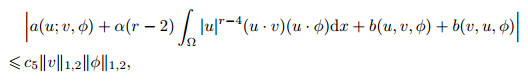
Proof   In actuality, we simply need to prove a priori estimate of the pressure p. Using Lemma 1, for all (u, p)∈ X× M, we have

From the above inequality, if we can estimate the quasi-bilinear a(u; u, v), the estimate of p is clear. Note that, if u ∈ L^r(Ω), then |u|^r-2u ∈ L^r'(Ω), where 1/r+1/r'=1, and we also have ‖|u|^r-2u‖_{0, r'}=‖u‖_{0, r}^r-1. Thus, we obtain

Finally, by combining the above inequalities with (6), the estimate of p is obtained.

Next, the estimation dependency of the Forchheimer coefficient α enables us to look into the behavior of the solutions as α tends toward zero. Let us use u_α to denote the solution to Problem (P) as α≠ 0, and u(0) to denote the solution to the Navier-Stokes equations, that is, Problem (P) with α=0.

Theorem 3    Assume that f ∈ X'. Then, u_α converges to u(0) in X as α tends toward zero. Moreover, if the condition (17) is satisfied, we have

(32)

Proof   u_α is the solution to Problem (P), that is,

(33)

Noting that , and by using Theorem 1, we obtain u^*∈ L²(Ω) such that

(34)

and

(35)

In contrast,

(36)

and ‖u‖_{0, r}≤ c₁‖u‖_{1, 2}. By applying Theorem 1, we obtain

Therefore,

(37)

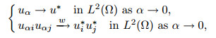
Hence, let α tend toward zero on both sides of Problem (P), and note that from Lemma 2 and (33)-(37), we obtain u^*, which equals the solution u(0) to Problem (P) as α=0 (that is, the Navier-Stokes equations), i.e.,

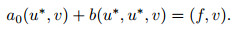
(38)

Using the difference between (33) and (38), and allowing v=u^*-u_α, we have

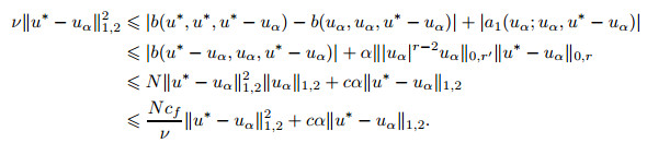
(39)

The conclusion to the theorem is obtained from the conditions in (17) and (39), and from the restriction of δ^*.

4 Finite element approximation 4.1 Existence and uniqueness of mixed element problem

For simplicity, we assume that Ω is a polygonal domain. Let a regular finite-element triangulation be given, where h is a discretization parameter that tends toward zero. Here, P_k denotes a kth-order polynomial. We introduce two finite dimensional spaces, W_h and Φ_h, such that

Then, we define the conforming finite element spaces X_h and M_h,

It is well known that the pair of finite element spaces X_h and M_h satisfies the discrete "LBB" condition, namely, there exists a constant independent of h such that

(40)

We also introduce the space

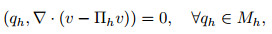
Corresponding to Problem (Q), we define the discrete problem (Q_h) as follows. Find (u_h, p_h)∈ X_h× M_h such that for all (v_h, q_h)∈ (X_h× M_h),

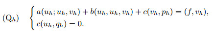
(41)

Similarly, Problem (P_h) is as follows. Find u_h ∈V_h such that for all v_h ∈ V_h,

(42)

Next, we define two new constants,

Under the hypotheses above, we have

(43)

Using the fixed point lemma^[27-28], we can prove the following theorem.

Theorem 4    Problem (P_h) has at least one solution u_h ∈ V_h, which satisfies

(44)

Moreover, Problem (P_h) has a unique solution u_h ∈ V_h provided that

(45)

Proof    For all v_h ∈ V_h, define the continuous mapping satisfying

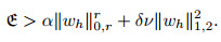
Allowing w_h= v_h, we then obtain

(46)

Thus, if

then

Hence, using the fixed point lemma, there exists an element u_h belonging to B(k)={u ∈ X, ‖u‖_X≤ k} such that

i.e., u_h is a solution to Problem (P_h). The estimation (44) can be obtained by setting v_h=u_h in Problem (P_h) and Lemma 1.

The proof of the uniqueness is similar and therefore omitted herein.

Next, let us prove the existence and uniqueness of Problem (Q). From Theorem 4, we only need to prove the uniqueness of p_h. Let us consider the functional defined on X_h, i.e.,

From Theorem 4, the space V_h is the null space of the functional , and noting that the discrete "LBB" condition in (40) is satisfied for (X_h, M_h), by using propositions 1.1 and 1.2 in Ref. [28], there exists a unique p_h ∈ M_h such that

i.e., (u_h, p_h) is a unique solution to Problem (Q_h). Therefore, the following theorem is proved.

Theorem 5    Problem (Q_h) has a unique solution (u_h, p_h)∈ X_h× M_h.

4.2 Error estimation

In this section, the approximation properties of the discrete problem can be deduced, where some hypotheses similar to the following have been introduced^[27-28].

Hypothesis H1    There exists an operator such that for some constant c>0, we have

(47)

and for 1≤ m≤ l,

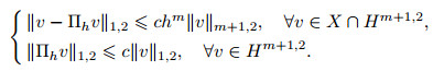
(48)

Hypothesis H2    There exists an operator such that for the constant c>0 and 1≤ m≤ l,

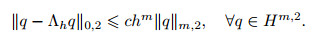
(49)

Next, we present the estimates for ‖u-u_h‖_{1, 2} and ‖p-p_h‖_{0, 2} in the following theorem.

Theorem 6    Assume that the solution (u, p) to Problem (Q) satisfies the regularity (u, p)∈ (X ∩ H^m+1)× (M ∩ H^{m, 2}), and that (u_h, p_h) is the solution to Problem (Q_h). There thus exists a constant c>0 such that

(50)

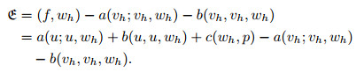
Proof    Let us first consider the error estimates of the velocity. Let v_h ∈ V_h be given, define w_h=u_h - v_h ∈ V_h, and consider the expression

(51)

Note that from (7), we have

Based on Lemma 1,

(52)

From the conclusion (43) and condition in (45), there exists δ>0 such that for all sufficiently small h>0,

(53)

and therefore from (52),

(54)

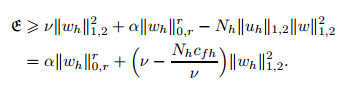
However, let us consider the upper bound for . From Problem (P_h), we have

(55)

It follows from (4) and (6)-(8) that

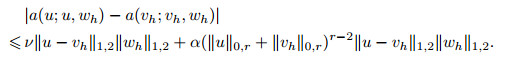
(56)

Thus,

(57)

In addition,

(58)

Combining the estimates to (54)-(58), we obtain

(59)

Finally, combining Theorems 1 and 2, hypothesis H1, and the triangular inequality, we obtain

(60)

Next, let us consider the error estimate of ‖p-p_h‖_M. From the discrete "LBB" condition in (40), ∀q_h ∈ M_h,

(61)

Clearly,

(62)

By using Problems (Q) and (Q_h), we have

(63)

where . From (61)-(63) and the triangle inequality, we have

(64)

Finally, by combining the hypotheses H1 and H2, (60), and (64), and selecting q_h=Λ_hp, the proof is complete.

5 Numerical iteration methods

In the previous section, the discrete approximation problem of a convective Brinkman-Forchheimer problem was presented, and some stability and error estimations were derived. By choosing explicit bases for X_h, V_h, and M_h, the discrete approximation problem can be converted into a nonlinear algebraic equation. In this section, several numerical iteration methods for a nonlinear algebraic system to solve the nonlinear algebraic equations are described. For simplicity, the iteration methods corresponding to Problem (P_h) will be generally considered, which can be easily expanded to Problem (Q_h).

5.1 Fixed point iteration

In general, the order of magnitude of the Forchheimer term is smaller than that of the other terms, and hence the explicit or semi-implicit discrete methodology can be used to approximate the Forchheimer term. In our opinion, when the viscosity is sufficiently large, the following fixed point iteration method will be effective, that is, for the given u_h⁽⁰⁾∈ V_h, find u_h⁽ⁿ⁾∈ V_h (n=1, 2, ...) such that

(65)

Clearly, there exists one and only one solution u_h⁽ⁿ⁾∈ V_h to (65).

5.2 Newton iteration

Let us first consider the nonlinear functional , which is constructed from the discrete approximation problem, i.e.,

(66)

The Newton iteration can then be defined as follows.

For the given u_h⁽⁰⁾∈ V_h, find u_h⁽ⁿ⁾∈ V_h (n=1, 2, ...) such that

(67)

where denotes the Gateaux derivative of at u along the direction w. Noting the definition of , (67) can be explicitly written as

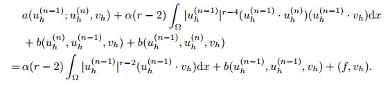
(68)

It is easy to prove that Problem (68) is uniquely solvable. For simplicity, let us omit the superscript (n) or (n-1) and the subscript h. Problem (68) is therefore equivalent to the following. For the given values u ∈ V_h and g ∈ V_h', find v ∈ V_h such that for all w ∈ V_h,

(69)

Theorem 7   Problem (69) has a unique solution, namely, v ∈ V_h.

Proof    In actuality, we only need to prove the continuity and elliptical property of the left-hand side of Problem (69). Let w=v in (69). From Theorem 1, we then have

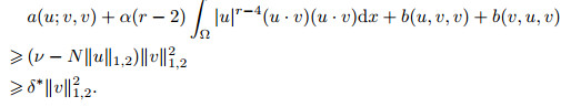
(70)

Next, if we denote I₁ and I₂ as

then

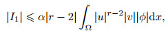
(71)

(72)

Noting that for all r ∈[2, ∞), , we then have

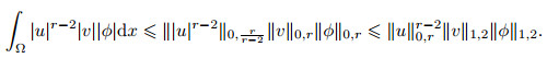
(73)

Hence, combining the inequality in (6), Theorem 2, and (71)-(73), we then have

(74)

where

Noting that V_h⊂ V, from (70) and (74), we can obtain the conclusion by using the Lax-Milgram theorem.

Note that, if the parameter 2 < r < 4, then the Newton iteration (68) may be singular. We also propose a semi-Newton iteration scheme, i.e.,

(75)

Clearly, there exists one and only one solution to the semi-Newton iteration scheme.

It is well known that the Newton iteration has a very high convergence rate if the initial value is properly selected. Therefore, we propose the following one-step Newton (or semi-Newton) iteration algorithm initialized through a fixed-point iteration, that is,

Step 1    Apply u_h⁽⁰⁾.

Step 2    Find u_h⁽ⁱ⁾(i=1, 2, ...) such that (65) is satisfied.

Step 3    Check the error ε=‖u_h⁽ⁱ⁾-u_h^(i-1)‖_{0, 2}.

(a) If , then return to Step 2.

(b) Otherwise, find u_h⁽ⁱ⁺¹⁾ such that (68) for r=2 and r≥4, or (75) for 2 < r < 4, is satisfied.

Step 4 Output the results.

6 Numerical examples

In this section, we present several numerical experiments on structured and unstructured triangular meshes through the conforming of a finite-element approximation. This investigation focuses on the validation of the convergence rate and the performances of the proposed methods, extending them to practical applications. Throughout this section, a Taylor-Hood element pair is used for discretization. We use the L² norm in the error control of the iterative algorithm, i.e.,

The GMRES solver is applied to solve the linear system obtained from a fixed-point iteration, and the conjugate-graduate method is used to solve the linear system obtained from the Newton or semi-Newton iteration.

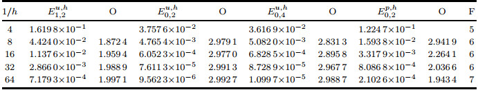
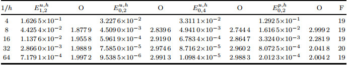
We test Examples 1 and 2 to show the convergence of the iterative algorithm based on the different parameters selected. Let r≥ 2, and

denote the relative errors in the tables. We set ν=1 and ε=10^-12 in Examples 1 and 2, and set ν=1/100, 1/400 and ε=0.5×10^-6 in Example 3. The results are as follows.

Example 1   Structured triangular mesh

Let Ω=[0, 1]×[0, 1], and be a given structured triangular mesh of Ω with a mesh size of h. A typical mesh is shown in Fig. 1(a). In this example, (u₁, u₂, p) is the analytical solution to the problem, i.e.,

When r=2, 3, 4 and α=1, 10, 100, the numerical errors with regard to the velocity and pressure, and the number of fixed-point iterations, are reported in Tables 1-9. It is easy to see that the convergence rate is consistent with the theoretical results. From Tables 3, 6, and 9, we can see that for a large Forchheimer coefficient α=100, the computation requires more fixed-point iterations to achieve the given accuracy with an increase in nonlinearity, i.e., r=2, 3, 4.

Example 2    Unstructured triangular mesh

Let Ω=[0, 1]×[0, 1], and be a given structured triangular mesh of Ω with a mesh size of h =h_max =(h₁, h₂, h₃, h₄, h₅), in which

A typical mesh is shown in Fig. 1(b). In this example, (u₁, u₂, p) is the analytical solution to the problem, i.e.,

where c=10. When r=2, 3, 4 and α=1×10^-3, the results are listed in Tables 10-12. We can see that the numerical results agree with the theoretical results.

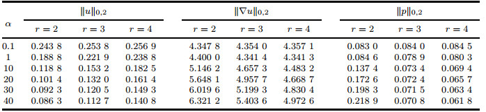
Example 3    Lid-driven problem

The lid-driven problem seeks the incompressible steady plane flow of a viscous fluid in a unit-square domain whose lid drives the flow by moving parallel to itself at a fixed speed. To display the different flow properties between the convective Brinkman-Forchheimer equations and the Navier-Stokes equations, we conduct some numerical tests using the convective Brinkman-Forchheimer equations under the lid-driven conditions, and compare our numerical results with the standard conclusion of a lid-driven cavity flow for the Navier-Stokes equations, for example, that by Ghia et al.^[32]. Herein, we set the boundary conditions as v = 0 on four sides, u = 0 on three sides, and u = 1 on the lid. In this example, the unstructured triangular mesh is adopted with reference to Fig. 1(b).

We first compare the norms of the velocity and pressure for different values of parameters α and r, the results of which are reported in Table 13. From the data presented in Table 13, we can see the monotonicity of each norm with respect to the increase in α and r, which indicates that the monotone increases (or decreases) for a certain type of energy with respect to the coefficients α and r.

Next, the CPU time for different viscosities ν=1/100 and 1/400 is shown in Fig. 2, where α is set to 1. From Fig. 2, we can see that the magnitude of time consumption for r=3 and 4 is dramatically increased with respect to r=2 when the maximum mesh size is decreased. In actuality, we know that the magnitude of the velocity for a lid-driven flow increases quickly and reaches 1 on the lid, and that the nonlinear properties of term |u|^r-2u increase as r increases from 2 to 4. In addition, the factor |u|^r-2 is non-homogeneous in a fluid field. Therefore, the nonlinear property of the discrete algebraic equations corresponding to the convective Brinkman-Forchheimer is non-homogeneous and increases along with the increase in r. The above-mentioned point will change the diagonally dominant property of each equation in the discrete algebraic equations.

In Figs. 3 and 4, we present the contours of the velocity magnitude, pressure, and streamline pattern for different r and ν and fixed α=1. To compare the difference, the contours of the velocity magnitude and pressure with fixed values are plotted in the figures. From the graphs, we see that there is an apparent change in the velocity and pressure fields when the parameter r is increased.

From the contours of the velocity magnitude on the left side of Figs. 3 and 4, we can see that when r=2, the flow is mainly surrounding the neighboring area of the lid. However, along with an increase in r, i.e., r=3, 4, the flow is enhanced away from the lid part.

Based on the pressure contours in the middle of Figs. 3 and 4, we can see that the pressure field changes from a layered structure to a complex structure with an increase in r.

From the streamline patterns on the right side in Figs. 3 and 4, we can see that with an increase in r, the location of the primary vortex deviates from the lid and right-side boundary, and approaches the geometric center of the flow domain. Meanwhile, the height and width of the two-bottom vortexes increase, and the unsymmetrical aspect of the two-bottom vortexes is strengthened.

Finally, in Fig. 5, we compare the horizontal and vertical velocities with the results by Ghia et al.^[32]. We can clearly see from Fig. 5 that the distribution of the horizontal and/or vertical velocities along the geometric center of the convective Brinkman-Forchheimer equations approaches the corresponding components of the Navier-Stokes equations as the parameter r increases from 2 to 4. The thickness of the boundary layer near the bottom decreases with an increase in r. Meanwhile, the peak increases. The thickness of the boundary layer near the left and right boundaries remains approximately the same for different values of r, whereas the peaks increase with an increase in r. These conclusions are in accord with the results in Figs. 3 and 4.

7 Conclusions

This paper presents a mixed finite-element approximation of two-dimensional steady convective Brinkman-Forchheimer equations. The existence and uniqueness of the variational problem and conforming finite-element approximation are proved. In addition, the order of convergence and error estimates are analyzed. Finally, a one-step Newton (or semi-Newton) iteration algorithm initialized using a fixed-point iteration is proposed. Numerical experiments using a Taylor-Hood mixed element built on a structured or unstructured triangular mesh are implemented. The numerical results of the lid-driven problem show that the energy of the fluid flow, corresponding to a different norm of the velocity u and pressure p, exhibits a monotone property with respect to the coefficients α and r. Meanwhile, for a fixed coefficient α=1, the flow patterns of the convective Brinkman-Forchheimer equations tend to agree with the Navier-Stokes equations with an increase in r.

Acknowledgements  This work was supported through a research fund from the Key Laboratory of Xinjiang Uygur Autonomous Region of China (No. 2017D04030). We thank the editor and anonymous referees for their careful reading of the manuscript and for their suggestions, which helped us improve the overall presentation of the paper.